6. Examples

6.1. Poiseuille Flow

We define the simulation domain for the Lattice Boltzmann Method (LBM). In this example, we choose a resolution of 30×30×30. Periodic boundary conditions are applied along the XX and YY axes, while the ZZ axis remains non-periodic.

do_domain:
  - domain:
     bounds:    [ [0,0,0] , [0.1,0.1,0.1] ]
     cell_dims: [ 30 , 30 , 30 ]
     periodic:  [ true, true, false ]

We apply a Neumann boundary condition on both Z boundaries at once, via the regions parameter (setting to (ux = 0, uy = 0, uz = 0)):

boundary_conditions:
  - neumann:
     U: [0.0,0,0]
     regions: [plan_xy_0, plan_xy_l]

An external force of (9.512485×10−5,0.0,0.0) is applied to drive the flow. The kinematic viscosity is set to 1e−3, and the average density is assumed to be 1000.

set_lbm_parameters:
  - lbm_parameters:
     Fext: [9.512485e-05,0.000000e+00,0.000000e+00]
     nuth: 1e-3

A plot_line_velocity analysis operator samples the velocity along a line probe at the center of the domain every 300 iterations. A plane_velocity_profile checker also exports the average Z profile:

analysis:
  - plot_line_velocity:
     line: [[0.05,0.05,0],[0.05,0.05,0.1]]

checker:
  - plane_velocity_profile:
     dimension: Z

global:
   simulation_paraview_freq: 100
   simulation_analysis_freq: 300
   simulation_end_iteration: 3000

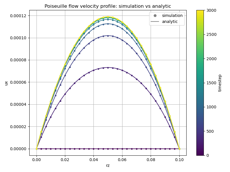
The expected results should show the development of a fully developed Poiseuille flow profile along the Z axis, with velocity increasing towards the center and decreasing near the boundaries due to the imposed Neumann conditions.

The velocity profile along Z, compared against the analytical transient Poiseuille solution, can be plotted using the provided post-processing script:

python3 ../hippoLBM/script/profile/plot_line_poiseuille.py PoiseuilleTestDir/Profile

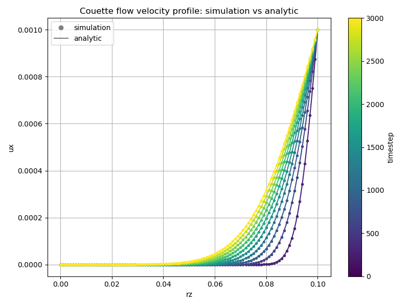
6.2. Couette Flow

We define the simulation domain for the Couette flow using the Lattice Boltzmann Method (LBM). In this case, we set the resolution to 100×100×100, with periodic boundary conditions applied on the XX and YY axes, and non-periodic boundary on the ZZ axis.

do_domain:
  - domain:
     bounds: [[0,0,0],[0.1 m,0.1 m,0.1 m]]
     cell_dims: [ 100 , 100 , 100 ]
     periodic: [true, true, false]

We set the Lattice Boltzmann parameters with a kinematic viscosity (nuth) of 1e-3 m2/s, a relaxation time tau of 0.7, and no external force applied (i.e., Fext = [0, 0, 0]).

set_lbm_parameters:
  - lbm_parameters:
     Fext: [0,0,0]
     nuth: 1e-3  # m2/s
     tau: 0.7

A Neumann boundary condition is applied on the upper Z boundary (plan_xy_l), with the velocity set to U = [0.001, 0, 0], and a zero-velocity Neumann condition is applied on the lower Z boundary (plan_xy_0).

boundary_conditions:
  - neumann:
     U: [0.001,0,0]
     regions: [plan_xy_l]
  - neumann:
     U: [0,0,0]
     regions: [plan_xy_0]

Two analysis operators are configured: plane_velocity_profile exports the average velocity profile along Z, and plot_line_velocity samples the velocity along a line probe crossing the domain from Z = 0 to Z = 0.1. Both run every 300 iterations.

analysis:
  - plane_velocity_profile:
     dimension: Z
  - plot_line_velocity:
     line: [[0.05,0.05,0],[0.05,0.05,0.1]]

global:
   simulation_paraview_freq: 100
   simulation_analysis_freq: 300
   simulation_end_iteration: 3000

The expected results will show a linear velocity profile along the Z axis:

The velocity profile along the Z axis, once the flow is fully developed, can be plotted using the provided post-processing script:

python3 ../hippoLBM/script/profile/plot_line_couette.py CouetteTestDir/Profile --nu 1e-3 --dt 6.666667e-05

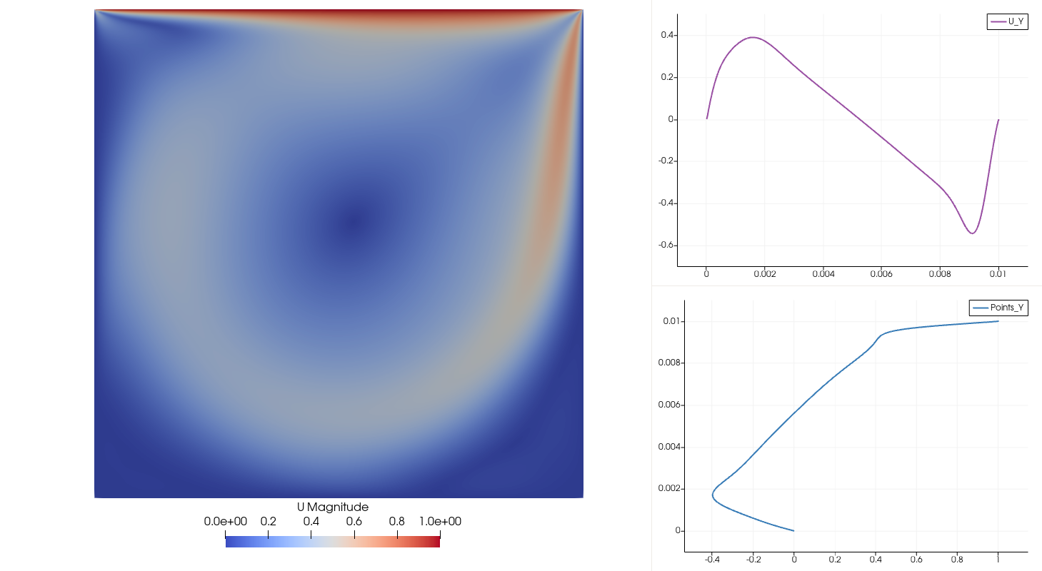
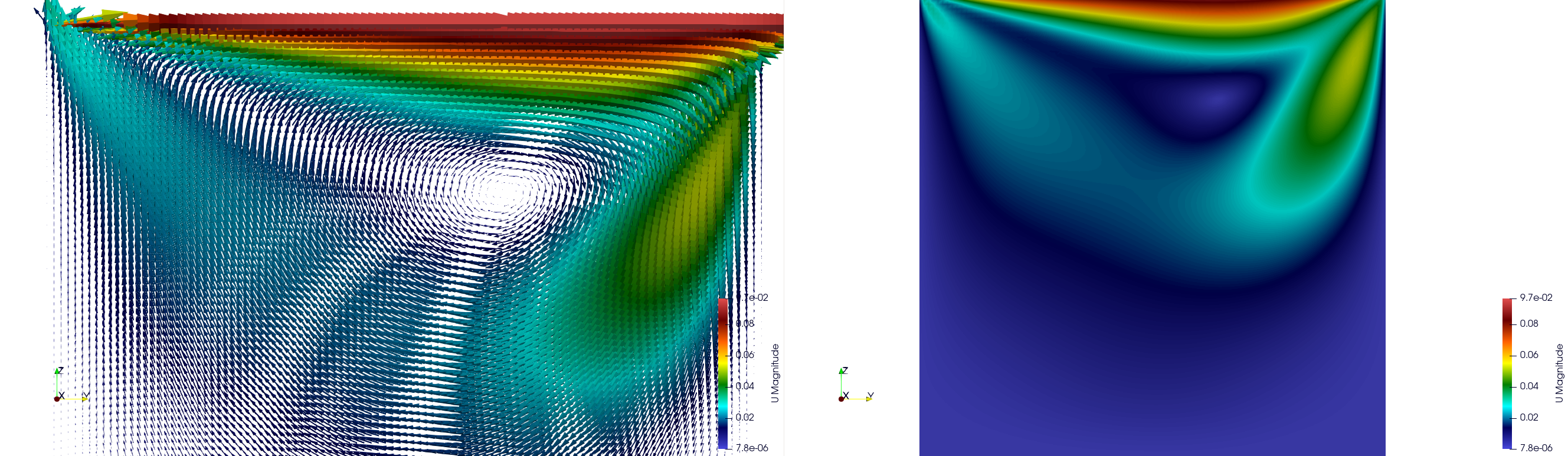
6.3. Lid-Driven Cavity Flow

This example simulates a lid-driven cavity flow using the Lattice Boltzmann Method (LBM), set up to reach a Reynolds number of 1000. The domain resolution is 400×10×400, with bounds expressed in meters, and periodic boundary conditions applied along the YY axis, and non-periodic boundaries on the XX and ZZ axes.

do_domain:
  - domain:
     bounds:    [ [0 m, 0 m, 0 m],[0.01 m, 0.00025 m, 0.01 m] ]
     cell_dims: [ 400 , 10 , 400 ]
     periodic:  [ false, true, false ]

No external force is applied (Fext = [0, 0, 0]), the kinematic viscosity is set to 1e-5 m2.s-1, the relaxation time tau is set to 0.7, and the celerity (speed of sound used to convert real units to LBM units) is set to 10.

set_lbm_parameters:
  - lbm_parameters:
     Fext: [0,0,0]
     nuth: 1e-5  # m2.s-1
     tau: 0.7
     celerity: 10

The collision model is set to BGK:

collision: bgk

Boundary conditions are applied using lid_driven_cavity in post_stream_bcs only. The moving lid with velocity U = [1, 0, 0] (Re = 1000) is applied on the upper XY plane (plan_xy_l). The three remaining non-periodic walls (plan_xy_0, plan_yz_0, plan_yz_l) are enforced as stationary walls by applying lid_driven_cavity with U = [0, 0, 0].

post_stream_bcs:
  - lid_driven_cavity:
     U: [1, 0.0, 0]  ## Re : 1000
     regions: [plan_xy_l]
  - lid_driven_cavity:
     U: [0, 0.0, 0]
     regions: [plan_xy_0, plan_yz_0, plan_yz_l]

The expected result is a recirculating vortex driven by the moving lid at the top of the cavity, characteristic of the classical lid-driven cavity benchmark.

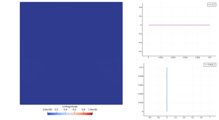
The velocity field once the flow has reached its steady state is shown below:

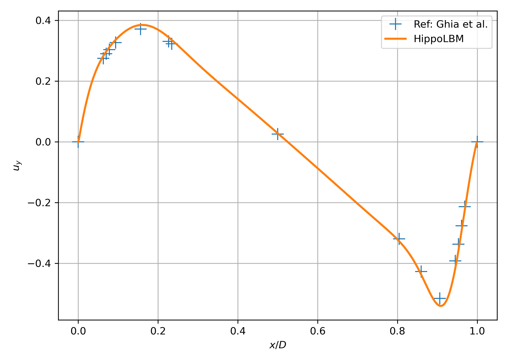
The centerline velocity profiles compared against the reference data of [4] are shown below:

6.4. Karman Vortex Street

This example simulates flow past a spherical obstacle using the Lattice Boltzmann Method (LBM). A body force drives the flow along the X axis. The domain is periodic in XX and YY, with non-periodic boundaries on the ZZ axis.

do_domain:
  - domain:
     bounds: [[0,0,0],[1.0,0.2,0.3]]
     cell_dims: [ 800, 160, 240 ]
     periodic: [true, true, false]

A body force of 1.3 along X drives the flow. The kinematic viscosity is 1e-3 and the relaxation time tau is set to 0.65.

set_lbm_parameters:
  - lbm_parameters:
     Fext: [1.3, 0.0, 0.0]
     nuth: 1e-3
     tau: 0.65

The collision model is BGK:

collision: bgk

A spherical obstacle is placed off-center in the domain:

set_obstacles:
  - register_solid_ball:
     id: 0
     center: [0.1001, 0.1027, 0.15023]
     radius: 0.03

Neumann zero-velocity conditions are applied on both ZZ boundaries, and wall bounce-back handles the obstacle surface:

boundary_conditions:
  - neumann:
     U: [0,0,0]
     regions: [plan_xy_0, plan_xy_l]

pre_stream_bcs:
  - wall_bounce_back

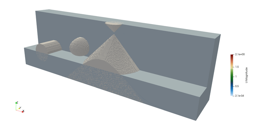
6.5. Flow Around Parametric Shapes

This example illustrates the use of quadric surfaces to define obstacles using the register_quadrics operator. Three shapes (cylinder, sphere, cone) are placed in the domain. The flow is driven by a body force along X, with periodic boundary conditions along XX and YY axes.

do_domain:
  - domain:
     bounds: [[0,0,0],[1.0,0.2,0.3]]
     cell_dims: [ 400, 80, 120 ]
     periodic: [true, true, false]

An external force of 1.3 along X drives the flow. The kinematic viscosity is 1e-3, and the relaxation time tau is set to 0.65:

set_lbm_parameters:
  - lbm_parameters:
     Fext: [1.3, 0.0, 0.0]
     nuth: 1e-3
     tau: 0.65

The collision model is set to BGK:

collision: bgk

Three quadric obstacles are registered using register_quadrics. Each is defined by a named quadric type and a sequence of geometric transforms (scale then translate):

• cyly: cylinder aligned along the Y axis

• sphere: ellipsoid (sphere when scale is uniform)

• conez: cone aligned along the Z axis

set_obstacles:
  - register_quadrics:
     id: 0
     quadrics: cyly
     transform:
       - scale:     [ 0.05, 1,    0.05 ]
       - translate: [ 0.15, 0.1,  0.1  ]
  - register_quadrics:
     id: 1
     quadrics: sphere
     transform:
       - scale:     [ 0.05, 0.08, 0.05 ]
       - translate: [ 0.35, 0.1,  0.15 ]
  - register_quadrics:
     id: 2
     quadrics: conez
     transform:
       - scale:     [ 0.05, 0.05, 0.05 ]
       - translate: [ 0.55, 0.1,  0.25 ]

Neumann zero-velocity conditions are applied on both ZZ boundaries, and wall bounce-back is applied on obstacle surfaces:

boundary_conditions:
  - neumann:
     U: [0,0,0]
     regions: [plan_xy_0, plan_xy_l]

pre_stream_bcs:
  - wall_bounce_back

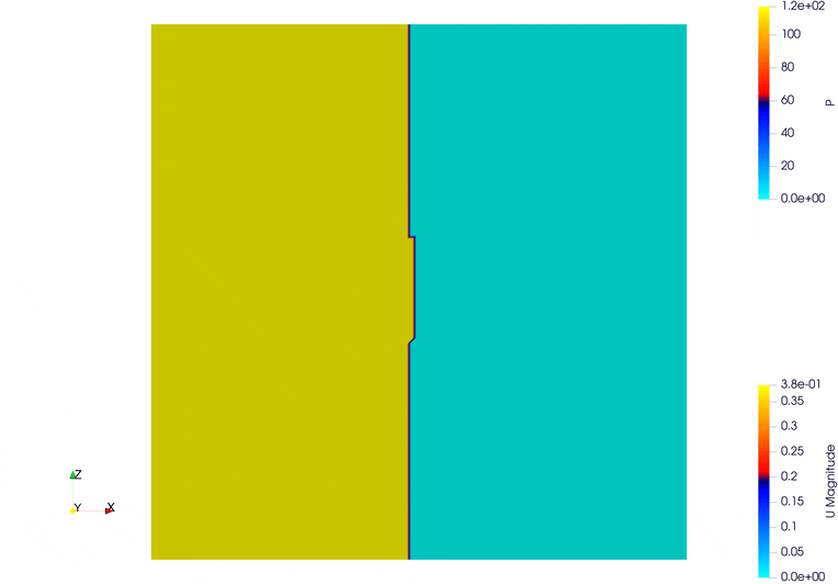
6.6. Pressure-Driven Flow

This simulation demonstrates the effect of a strong pressure or density difference using the Lattice Boltzmann Method (LBM). The domain has a resolution of 100×100×100, with periodic boundary conditions along the Y axis, and closed boundaries in X and Z.

do_domain:
  - domain:
     bounds:    [ [0,0,0] , [0.1,0.1,0.1] ]
     cell_dims: [ 100 , 100 , 100 ]
     periodic:  [ false, true, false ]

No external force is applied. The kinematic viscosity is set to 1e-4.

set_lbm_parameters:
  - lbm_parameters:
     Fext: [0.000000e+00,0.000000e+00,0.000000e+00]
     nuth: 1e-4

The pre-streaming boundary conditions include:

• pre_bounce_back: standard no-slip boundary on external walls.

• wall_bounce_back: bounce-back for internal structures.

pre_stream_bcs:
  - pre_bounce_back
  - wall_bounce_back

Two vertical internal walls are added near the center of the domain, one at the top and one at the bottom, leaving a gap in the middle. These walls obstruct flow and create more complex recirculation patterns.

set_obstacles:
  - register_solid_wall:
     id: 0
     bounds: [[0.048,0,0.06],[0.052,0.1,0.1]]
  - register_solid_wall:
     id: 1
     bounds: [[0.048,0,0],[0.052,0.1,0.04]]

A high-density region is initialized on the left-hand side using set_distribution with a coefficient of 1.5. This creates a pressure difference between the left and right sides of the domain, acting as the flow-driving mechanism.

set_distributions:
  - set_distribution:
     value: 1.5
     bounds: [[0,0,0], [0.048,1,1]]

Warning

The value parameter is applied uniformly to all distribution function components \(f_i\). This is a raw initialization of the distributions, not a thermodynamically consistent density initialization.

The post-streaming boundary condition is the standard post_bounce_back.

post_stream_bcs:
  - post_bounce_back

The goal of this setup is to observe how a sharp pressure gradient (from the initialized distribution) drives flow across the domain.

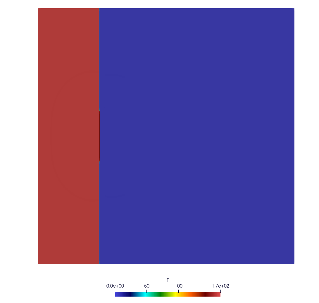
6.7. Pressure-Driven Flow Through Complex Geometry

This simulation demonstrates pressure-driven flow across a complex internal structure using the Lattice Boltzmann Method (LBM). The domain is discretized with a resolution of 400×400×400, offering fine detail of the flow field. Periodic boundary conditions are applied along the Y axis, and the X and Z axes remain non-periodic.

do_domain:
  - domain:
     bounds:    [ [0,0,0] , [0.1,0.1,0.1] ]
     cell_dims: [ 400 , 400 , 400 ]
     periodic:  [false, true, false ]

No external force is applied (Fext = [0,0,0]), and the kinematic viscosity is set to 1e-4.

set_lbm_parameters:
  - lbm_parameters:
     Fext: [0,0,0]
     nuth: 1e-4

Pre-streaming boundary conditions include bounce-back on all walls and user-defined internal walls:

pre_stream_bcs:
  - pre_bounce_back
  - wall_bounce_back

A complex system of internal obstacles (walls) is defined to create a tortuous path for the flow. These walls are strategically placed along the X axis to create narrow channels and mixing zones.

set_obstacles:
  - register_solid_wall:
     id: 0
     bounds: [[0.024,0,0.06],[0.026,0.1,0.1]]
  - register_solid_wall:
     id: 1
     bounds: [[0.024,0,0],[0.026,0.1,0.04]]
  - register_solid_wall:
     id: 2
     bounds: [[0.034,0,0.025],[0.036,0.1,0.075]]
  - register_solid_wall:
     id: 3
     bounds: [[0.049,0,0.06],[0.051,0.1,0.1]]
  - register_solid_wall:
     id: 4
     bounds: [[0.049,0,0],[0.051,0.1,0.04]]
  - register_solid_wall:
     id: 5
     bounds: [[0.068,0,0.0355],[0.072,0.1,0.065]]
  - register_solid_wall:
     id: 6
     bounds: [[0.085,0,0.02],[0.1,0.1,0.03]]
  - register_solid_wall:
     id: 7
     bounds: [[0.085,0,0.07],[0.1,0.1,0.08]]

A high-density initialization is imposed on the far left of the domain using set_distribution with a value of 1.5. This sets up a large pressure difference that drives the fluid flow.

set_distributions:
  - set_distribution:
     value: 1.5
     bounds: [[0,0,0], [0.024,1,1]]

Warning

The value parameter is applied uniformly to all distribution function components \(f_i\). This is a raw initialization of the distributions, not a thermodynamically consistent density initialization.

Post-streaming bounce-back is applied to maintain no-slip conditions at the boundaries:

post_stream_bcs:
  - post_bounce_back

6.8. Cavity Flow [OLD]

We define the simulation domain for the cavity flow using the Lattice Boltzmann Method (LBM). In this case, the resolution is set to 200×200×200, with non-periodic boundary conditions applied in all directions (XX, YY, and ZZ).

do_domain:
  - domain:
     bounds:    [ [0,0,0] , [0.1,0.1,0.1] ]
     cell_dims: [ 200 , 200 , 200 ]
     periodic:  [ false, false, false ]

We set the Lattice Boltzmann parameters, with no external force applied (i.e., Fext = [0, 0, 0]) and a kinematic viscosity (nuth) of 1e-4.

set_lbm_parameters:
  - lbm_parameters:
     Fext: [0.000000e+00,0.000000e+00,0.000000e+00]
     nuth: 1e-4

The boundary conditions for the simulation are defined as follows:

• Pre-streaming boundary conditions: The pre_bounce_back and cavity_z_l conditions are set, with a velocity of U = [0.0, 0.1, 0] applied on the lower Z boundary.

• Post-streaming boundary condition: The post_bounce_back condition is applied on the other boundaries.

pre_stream_bcs:
  - pre_bounce_back
  - cavity_z_l:
     U: [0.0, 0.1, 0]

post_stream_bcs:
  - post_bounce_back

The expected results will show the development of a cavity flow pattern, where the fluid moves along the Z axis, influenced by the velocity set on the lower boundary. This is typical for cavity simulations, where the fluid is confined within a box.

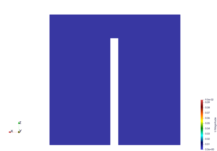
6.9. Cavity Flow with Wall Obstacle [OLD]

This example simulates cavity flow using the Lattice Boltzmann Method (LBM) with a fixed obstacle (wall) in the middle of the domain. The domain resolution is 100×100×100, and non-periodic boundary conditions are enforced on all axes (XX, YY, and ZZ).

do_domain:
  - domain:
     bounds:    [ [0,0,0] , [0.1,0.1,0.1] ]
     cell_dims: [ 100 , 100 , 100 ]
     periodic:  [ false, false, false ]

No external force is applied (Fext = [0, 0, 0]), and the kinematic viscosity is set to 1e-4.

set_lbm_parameters:
  - lbm_parameters:
     Fext: [0.000000e+00,0.000000e+00,0.000000e+00]
     nuth: 1e-4

Boundary conditions are applied as follows:

• Pre-streaming:

  • pre_bounce_back applies bounce-back on walls.

  • cavity_z_l sets a moving lid on the lower Z boundary with velocity U = [0.1, 0.0, 0].

  • wall_bounce_back enables bounce-back condition for the internal obstacle.

• Post-streaming:

  • post_bounce_back finalizes bounce-back conditions after streaming.

pre_stream_bcs:
  - pre_bounce_back
  - cavity_z_l:
     U: [0.1, 0.0, 0]
  - wall_bounce_back

post_stream_bcs:
  - post_bounce_back

An internal obstacle is defined using the set_obstacles field. A vertical wall is placed at the center of the domain, slightly offset in the X-direction, spanning from Z = 0 to Z = 0.08.

set_obstacles:
  - register_solid_wall:
     id: 0
     bounds: [[0.048,0,0],[0.052,0.1,0.08]]

The expected result is a modified cavity flow field with recirculation zones forming around the central wall obstacle, demonstrating how internal structures influence fluid dynamics in confined spaces.