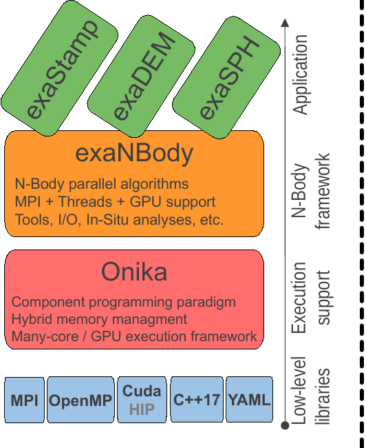
1. ExaNBody: Framework for N-Body Simulations on HPC Platforms
This framework, developed at the French Atomic Agency (CEA), is tailored for N-Body simulations on High-Performance Computing (HPC) platforms. Originally designed for the ExaSTAMP Molecular Dynamics code, it has been extended to cater to various N-Body problems.
Key Characteristics:
Language: Implemented in C++17, leveraging modern language features for efficiency and versatility.
- Parallelization:: Hybrid approach integrating:
Vectorization for CPU optimization.
Thread-parallelization using OpenMP for multi-core architectures.
GPU-parallelization via CUDA to harness GPU computational power.
MPI-parallelization for distributed memory systems.
Spatial Domain Decomposition: Utilizes spatial domain decomposition techniques for efficient workload distribution among processors.
Load Balancing (RCB): Implements Load Balancing using Recursive Coordinate Bisection (RCB) for optimal task distribution among processing units.
Parallel IO: Enables efficient handling of parallel Input/Output operations. Supports checkpoint files, parallel Paraview files, and diagnostics in a parallelized manner.
In-situ Analysis: Provides real-time data analysis capabilities during simulation execution, minimizing data movement and storage overhead.
1.1. ExaDEM Variant
ExaDEM is a software solution in the field of computational simulations. It’s a Discrete Element Method (DEM) code developed within the exaNBody framework. This framework provides the basis for DEM functionalities and performance optimizations. A notable aspect of ExaDEM is its hybrid parallelization approach, which combines the use of MPI (Message Passing Interface) and Threads (OpenMP). This combination aims to enhance computation times for simulations, making them more efficient and manageable.
Additionally, ExaDEM offers compatibility with MPI``+``GPUs, using the CUDA programming model (Onika layer). This feature provides the option to leverage GPU processing power for potential performance gains in simulations. Written in C++17, ExaDEM is built on a contemporary codebase. It aims to provide researchers and engineers with a tool for adressing DEM simulations.
1.2. ExaSPH Variant
1.3. ExaSTAMP Variant
2. Installing ExaNB
To proceed with the installation, your system must meet the minimum prerequisites. The first step involves the installation of exaNBody:
git clone https://github.com/Collab4exaNBody/exaNBody.git
mkdir build-exaNBody/ && cd build-exaNBody/
cmake ../exaNBody/ -DCMAKE_INSTALL_PREFIX=path_to_install
make install
export exaNBody_DIR=path_to_install
3. N-Body Background
3.1. N-body methods
N-body methods encompass a variety of techniques used to model the behavior and interactions of a set of particles over time. These methods consist in solving Newton’s equation of motion f = ma for each particle at each time step, where f corresponds to the sum of the forces applied to the particle, a its acceleration and m its mass. The forces are deduced from the interactions between particles according to their types, i.e. contact, short-range, or long-range interactions, and external forces applied to the sample (i.e. gravity). Velocities are then deduced from the accelerations and subsequently used to update the particle positions at the next time step. This process is repeated, typically with a fixed time step ∆t, according to an integration scheme4 until the desired duration is reached. The collection of particle configurations over time allows to study a wide range of phenomena, from granular media movements, with the Discrete Element Method (Dem), to material crystal plasticity at the atomic scale using Molecular Dynamics (Md), going up to the galaxy formation with the Smoothed-Particle Hydrodynamics (Sph).
3.2. N-body simulation codes
The development of a N-body code is led by the need to figure out the neighborhood of a given particle for every timestep in order to process interactions of different kinds.
Particle interactions can be categorized as short-range and long-range. Short-range interactions are considered negligible beyond a specified cut-off radius. To optimize calculations, neighboring particle detection algorithms are employed to eliminate unnecessary computations with distant particles. Each N-Body method employs a wide variety of short-range interactions that capture different particle physics. For example, visco-elastic contacts in Discret Element Method follow Hooke’s law or Hertz law to model contact elasticity between rigid particles, while pair potentials like Lennard-Jones or Morse are used for gas or liquid atom interactions in classical Md. Long-range interactions, on the other hand, can sometimes not be neglected and result in algorithmic complexity of O(N 2 ). Such interactions, like gravitation in astrophysics, or electrostatic forces in Molecular Dynamics, are typically modeled using the Ewald summation method. Fortunately, calculation approaches such as the fast multipole method can achieve a complexity of O(N ), thanks to an octree structure, and can be efficiently parallelized. Although this paper primarily focuses on short-range interactions, both types of interaction can be dealt with in exaNBody.
Neighbor lists are built, using different strategies, to shorten the process of finding out the neighbors of a particle within the simulation domain. It helps optimizing the default algorithm having a complexity of O(N^2) that tests every pair of particles (if N is the number of particles). The most common strategy to deal with any kind of simulation (static or dynamic, homogeneous and heterogeneous density) is a fusion between the linked-cell method, see figure 2, and the Verlet list, see figure 2 method. The combination of these methods has a complexity of O(N) and a refresh rate that depends on the displacement of the fastest particle. This algorithm is easily thread-parallelized. Others less-used neighbor search strategies have been developed to address specific simulations
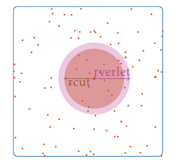
Figure 1: A method for building neighbor lists using the Verlet lists. rcut is the radius cut-off and rVerlet is the radius of Verlet.
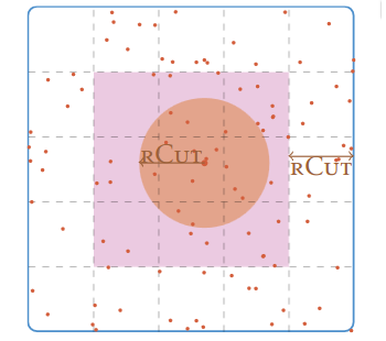
Figure 2: A method for building neighbor lists using linked cells. rcut is the radius cut-off.
Domain decomposition is usually employed in N-Body methods to address distributed memory parallelization, assigning one subdomain to each MPI process. This implies the addition of ghost areas (replicated particles) around subdomains to ensure each particle has access to its neighborhood. Over time, many algorithms have been designed to improve load-balancing such as: Recursive Coordinate Bisection (RCB), the Recursive Inertial Bisection (RIB), the Space Filling Curve (SFC), or graph method with ParMETIS. Note that the library Zoltan gathers the most popular methods. To ease neighbor list construction (i.e. employing the linked-cell method), the simulation domain is described as a cartesian grid of cells, each of which containing embedded particles. Each subdomain then consists in a grid of entire cells assigned to one Mpi process. In contrast, concurent iteration over the cells of one subdomain’s grid provides the basis for thread parallelization at the NUMA node level.
Commonalities are shared across N-body simulation codes, such as numerical schemes, neighbor particle detection, or short/long-range interactions. The computation time dedicated to interaction and force calculations can be significant (over 80% of the total time) depending on the studied hpenomenon complexity. Additional factors, such as neighbor lists construction computational cost, can impact overall simulation time. For dynamic simulations involving rapidly moving particles and computationally inexpensive interactions, more than 50% of the total time may be spent on neighbor list construction. The computationally intensive sections of the code vary depending on methods and phenomena studied, requiring optimizations such as:
MPI parallelization
Vectorization
Multi-threading
GPU usage
4. Software stack of ExaNBody
4.1. Software Stack Layers:
External Libraries: This layer encompasses external dependencies utilized by the software. These libraries are leveraged to access functionalities that are not internally developed, enhancing the overall capabilities of the system.
HPC Libraries: High-Performance Computing (HPC) libraries serve as powerful tools within the software stack, providing optimized routines and functionalities specifically designed for high-computational tasks.
Low-Level and Runtime Support (Onika): Foundational infrastructure and runtime support are provided by this layer. Onika serves as the backbone, offering essential utilities for the execution and management of the software. It’s important to note that ongoing efforts are directed towards integrating frameworks like OpenMP or CUDA.
N-Body Framework: Positioned at the core of the software stack, the N-Body Framework proposes a large variety of N-Body features to build efficiently N-Body simulation such as traditionnal integration schemes, IO, or partiionning methods.
Application Layer: This layer encapsulates the specific applications built upon the software stack. It provides the interface for users to interact with the functionalities offered by the stack and serves as the platform for N-Body application-specific implementations and functionalities.
4.2. Guidelines for operators:
Common Operators: These operators serve as N-Body fundamental operations utilized across various components of the software, facilitating consistent functionality and reducing redundancy.
Application-Specific Operators: Tailored operators designed to cater to the unique requirements of specific applications built on top of the software stack.
Mutualization: This process involves the consolidation and centralization of specific operators shared by multiple applications. It aims to optimize resources and streamline the execution of these shared functionalities.
Specific Operators Shared Among Applications: For increased efficiency and ease of access, specific operators that are shared among multiple applications are centralized within exaNBody. This consolidation not only ensures optimized utilization but also simplifies management and maintenance, benefiting all associated applications.
5. Performance and portability
The complex and ever-changing architectures of modern supercomputers make it difficult to maintain software performance. exaNBody aims at providing performance portability and sustainability on those supercomputers with robust domain decomposition, automated inter-process communications algorithms, adaptable particle data layout, and a set of hybrid (CPU/GPU) parallelization templates specialized for N-Body problems.
5.1. Application level specialization
First of all, the internal units to be used are specified as well as the physical quantities to be stored as particle attributes. These quantities (or fields), are defined using a symbolic name associated with a type, e.g. velocity as a 3D vector. A field set is a collection of declared fields. One of the available field sets is selected and used at runtime, depending on simulation specific needs. As depicted in figure below, particles are dispatched in cells of a cartesian grid spanning the simulation domain. In short, the data structure containing all particles’ data will be shaped as a cartesian grid of cells, each cell containing all fields for all particles it (geometrically) contains. More specifically, the reason why fields and field sets are defined at compile time is that particle data storage at the cell level is handled via a specific structure guaranteeing access performance and low memory footprint.
5.2. Spatial domain decomposition and inter-process communications
The coarsest parallelization level can become the main bottleneck due to network latencies and load imbalance issues. To take advantage of this first level of parallelization, the simulation domain is divided into subdomains using an recursive coordinate bisection (RCB) algorithm, as depicted in figure below, assigning one subdomain to each MPI process.
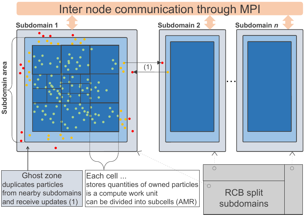
Figure 1: Overview of domain decomposition and inter process communications in exaNBody framework.
This is achieved thanks to three main components: cell cost estimator, RCB domain decomposition, and particle migration. Particle migration can be used as-is by any N-Body application, thanks to the underlying generic particle data storage. It supportsheavily multi-threaded, large scale, simulations while lowering peak memory usage. Additionally, the migration algorithm is also customizable to fit specific application needs, keeping unchanged the core implementation. For instance, molecualr dynamics simulations may transport per-cell data fields and discret element method simulations may migrate friction information related to pair of particles. Finally, ghost particle updates are available to any N-Body application, via customizable components.
5.3. Intra-node parallelization API
This API is available in exaNBody to help developers express parallel computations within a MPI process. This API offers a set of parallelization templates associated with three types of computation kernels:
Local calculations on a particle (such as resetting force operator)
calculations coupled with reduction across all particles (such as getting the total number of particles or the current temperature)
calculations involving each particle and its neighbors (such as computing potential forces in molecular dynamics or contact forces in discret element method)
When a developer injects a compute function into these templates, computation may be routed to CPU or GPU, as illustrated in figure below.
Figure 2: Example of a particle centered computation executable on both COU and GPU. Three ingredients: a user functor (the kernel), static execution properties (via traits specialization), a ready to use parallelization function template.
While thread parallelization on the CPU is powered by OpenMP, Cuda is employed to execute the computation kernel on the Gpu, using the same provided function. The main difference between the two execution modes is that each cell is a unitary work unit for a single thread in OpenMP context but it is processed by a block of threads in Cuda. Those two parallelization levels (multi-core and GPU) are easily accessible to developers thanks to the execution support layer of Onika. Onika is the low-level software interface that powers exaNBody building blocks. It is responsible for aforementioned data containers, memory management (unified with GPU), and it is the foundation for hybrid execution abstraction layer.
5.4. Particle data layout and auxiliary data structures
These two points are two essential features to maximize performance at the NUMA node level. In exaNBody, particle data are packed independently in each cell using a container specifically designed to match both CPU’s SIMD and GPU’s thread blocks requirements concerning data alignment and vectorization friendly padding. This generic container, available in ONIKA toolbox, not only adapts to specific hardware characteristics at compile time, but ensures minimal memory footprint with as low as 16 bytes overhead per cell regardless of the number of data fields, allowing for very large and sparse simulation domains. N-Body simulations also heavily depend on particles’ neighbors search algorithm and storage structure. The search usually leverages the grid of cell structure to speed up the process, and neighbors lists data structure holds information during several iterations. However, depending on the simulation, particles may move rapidly while their distribution may be heterogeneously dense. Those two factors respectively impact neighbor list update frequency and its memory footprint. On the one hand, exaNBody takes advantage of an Adaptive Mesh Refinement (AMR) grid to accelerate (frequent) neighbor list reconstructions. On the other hand, a compressed neighbor list data structure saves up to 80% of memory (compared to uncompressed lists) while still ensuring fast access from both the CPU and the GPU.
5.5. Flexible and user friendly construction of N-Body simulations
A crucial aspect for software sustainability is to maintain performance over time while managing software complexity and evolution. Complex and rapidly evolving scientific software often encounter common pitfalls, such as code duplication, uncontrolled increase in software inter-dependencies, and obscure data/control flows. This observation has led us to develop our component-based model to avoid these pitfalls. In our model, individual software components are implemented using C++17 and are application structure oblivious, meaning they only know their input and output data flows. Application obliviousness is a crucial aspect of the present design, promoting reusability while preventing uncontrolled growth of internal software dependencies. Each component is developed as a class, inheriting from a base class OperatorNode and explicitly declares its input and output slots (data flow connection points). Once compiled, these components are hierarchically assembled at runtime using a Sequential Task Flow (STF), with a YAML syntax, as shown in figure below.
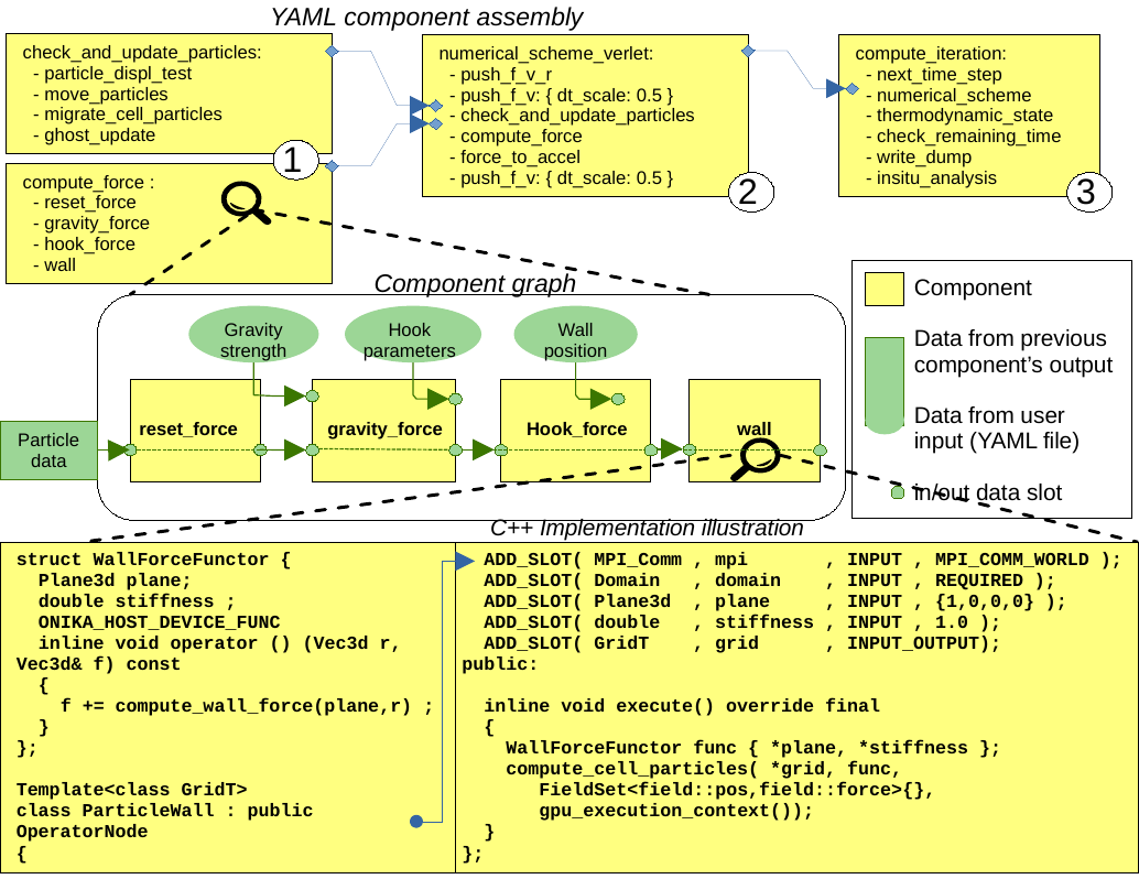
Figure 3: Illustrative sample of components assembly using YAML description. 1) C++ developed components are assembled and connected in the manner of a STF, creating a batch component. 2) and 3) illustrate batch components aggregation to higher and higher level components, up to full simulation task flow.
A set of base components are already available to developers, embedded within exaNBody, such as: common computations, checkpoint/restart, visualization and In-Situ analytics, allowing developers to focus on their application specific components. We also observed that this component based approach not only prevents some development pitfalls, but enables various simulation code structures. YAML formatted component configuration makes it simple for a user to amend or fine tune the simulation process. For instance it can be used to change the numerical scheme or even to insert In-Situ analysis components at specific stages of the simulation process, leveraging In-Situ processing to limit disk I/O. Finally, this component based splitting of the code gives exaNBody the opportunity to provide integrated profiling features that automatically give meaningful performance metrics for each part of the simulation. It allows the user to access computation time spent on CPU and GPU, as well as imbalance indicator. It can also interoperate with nSight System from NVIDIA and summarize memory footprint with detailed consumption.
6. Algorithm Patterns
This is Developer Documentation.
The aim of this section is to explain to developers the tools used in exaNBody to propose default parallel algorithms. For this purpose, we will describe the 4 main algorithmic patterns:
block_parallel_for: exposes a simple parallelization scheme (like a parallel for in OpenMP), but with a notion of “thread blocks” and the possibility of asynchronous execution. It is defined directly in the Onika layer, as it is not specific to particle systems.
compute_cell_particles: performs a parallel processing on all particles contained within a grid (Grid type pattern).
reduce_cell_particles: performs an operation on each particle returning a value, the values obtained being reduced to a single one (e.g., a sum).
compute_cell_particle_pairs: the most important and most used pattern, allows calculations on particles and their neighbors.
Guidelines:
Support hybrid execution, automatically directing calculations either to the CPU cores or to the GPU.
Avoid code duplication between components.
Avoid the complexities of setting up OpenMP/CUDA parallelism.
Allow asynchronous parallel operations (with results retrieved later in the code).
Automatically adapt to the different OpenMP parallelism modes supported by the component system (simple, nested, and task-based).
Facilitate the implementation of a single computation function for both CPU and GPU.
Manage dynamic load balancing among the SMs of the GPUs themselves.
6.1. Block Parallel For
This construction is the most rudimentary; it is equivalent to an OpenMP parallel for directive but with many additional possibilities. We will look at a step-by-step example where a fixed value is added to all elements of an array of arrays. The example on a two-dimensional array demonstrates the use of two-level multi-threaded parallelism we have discussed, which resembles a bit the array of cells, each containing a set of particles typically processed in exaNBody.
6.1.1. Basic usage
Before calling block_parallel_for, it is necessary to define the functor (the calculation function) that will be applied in parallel to our data.
namespace tutorial
{
  using namespace exanb;
  // a functor = function applied in parallel
  // it is defined by a class (or struct) with the call operator ()
  struct BlockParallelValueAddFunctor
  {
    Array2DReference m_array;
    double m_value_to_add = 0.0; // value to add
    ONIKA_HOST_DEVICE_FUNC            // works on CPU and GPU
    void operator () (size_t i) const // call operator with i in [0;n[
    {                                 // a whole block (all its threads) execute iteration i
      const size_t cols = m_array.columns();
      ONIKA_CU_BLOCK_SIMD_FOR(size_t, j, 0, cols)   // parallelization among the threads of the current block
      {                                             // for iterations on j in [0;columns[
        m_array[i][j] += m_value_to_add; // each thread executes 0, 1, or multiple iterations of j
      }
    }
  };
}
ONIKA_CU_BLOCK_SIMD_FOR: Defines a macro that facilitates the use of the second level of parallelism within threads of the same CUDA block.
Usage:
GPU :Ensures that the functor’s code is executed across all threads within a CUDA block with consistent iteration index i. When compiled for the GPU, it distributes iterations based on ONIKA_CU_BLOCK_SIZE and ONIKA_CU_THREAD_IDX.
CPU: On the host, this construct transforms into a straightforward for loop. However, on the host, the loop includes the OpenMP directive #pragma omp simd for, ensuring loop vectorization, even with only one CPU thread per block, provided CPU and compiler support is available.
Next, we need to inform the compiler whether our functor is compatible with CUDA. In some situations, our code may have a strong incompatibility (such as calling a non-compatible library) that would prevent it from compiling correctly with the nvcc layer. This needs to be known at compile time (not just at runtime) because otherwise, compilation errors would occur.
namespace onika
{
  namespace parallel
  {
    template<>
    struct BlockParallelForFunctorTraits<tutorial::BlockParallelValueAddFunctor>
    {
      static constexpr bool CudaCompatible = true; // or false to prevent the code from being compiled with CUDA
    };
  }
}
The final step is to launch the parallel operation in the code of our component:
namespace tutorial
{
  using namespace exanb;
  class SynchronousBlockParallelSample : public OperatorNode
  {
    ADD_SLOT(Array2D, my_array, INPUT_OUTPUT, REQUIRED);
    ADD_SLOT(double, my_value, INPUT, 1.0);
    public:
    inline void execute() override final
    {
      using onika::parallel::block_parallel_for;
      if( my_array->rows() == 0 || my_array->columns() == 0 )
      {
        my_array->resize( 1024 , 1024 );
      }
      BlockParallelValueAddFunctor value_add_func = { *my_array // refernce our data array through its pointer and size
                                                    , *my_value // value to add to the elements of the array
                                                    };
      // Launching the parallel operation, which can execute on GPU if the execution context allows
      block_parallel_for( my_array->rows()             // number of iterations, parallelize at the first level over rows
                        , value_add_func               // the function to call in parallel
                        , parallel_execution_context() // returns the parallel execution context associated with this component
                        );
    }
  };
}
The corresponding complete exemple is in exaNBody source tree and compiled, ready to be tested, and is linked here after : synchronous_block_parallel.cpp
6.1.2. Asynchronous parallel execution
In the following example, we are still using the simplest version of block_parallel_for, but we want to trigger parallel execution asynchrounsly (running in the background), and explicitly wait for completion later on. To this end, we capture object returned by block_parallel_for, of type ParallelExecutionWrapper, to handle its synchronization manually. When this object is not captured in a variable, it is therefor destructed right after termination of block_parallel_for, which has the side effect of launching and waiting for the completion of created parallel operation.
namespace tutorial
{
  class AsyncBlockParallelSample : public OperatorNode
  {
      ADD_SLOT(Array2D, my_array, INPUT, REQUIRED);
      ADD_SLOT(double, my_value, INPUT, 1.0);
  public:
    inline void execute() override final
    {
      using onika::parallel::block_parallel_for;
      if( my_array->rows() == 0 || my_array->columns() == 0 ) { my_array->resize( 1024 , 1024 ); }
      BlockParallelValueAddFunctor value_add_func = { *my_array // refernce our data array through its pointer and size
                                                  , *my_value // value to add to the elements of the array
                                                  };
      // Launching the parallel operation, which can execute on GPU if the execution context allows
      // result of parallel operation construct is captured into variable 'my_addition',
      // thus it can be scheduled in a stream queue for asynchronous execution rather than being executed right away
      auto my_addition = block_parallel_for( my_array->rows() // number of iterations, parallelize at the first level over rows
                                           , value_add_func   // the function to call in parallel
                                           , parallel_execution_context("my_add_kernel") // execution environment inherited from this OperatorNode
                                           ); // optionally, we may tag here ^^^ parallel operation for debugging/profiling purposes
      // my_addition is scheduled here, transfering its content/ownership (see std::move) to the default stream queue
      auto stream_control = parallel_execution_stream() << std::move(my_addition) ;
      lout << "Parallel operation is executing..." << std::endl;
      stream_control.wait();                               // wait for the operation to complete and results to be ready to read
      lout << "Parallel operation has completed !" << std::endl;
    }
  };
}
If the execution context allows it, the parallel operation will proceed in the background, occupying either the free threads (other than those executing this code) or the GPU. This can be very useful, especially for overlapping computations and MPI message sends. The corresponding complete exemple in exaNBody source tree is here : async_block_parallel.cpp
Warning
The operation is asynchronous only if the execution context permits it. Otherwise, it will proceed synchronously and complete before the block_parallel_for function returns. In such cases, calling control->wait() will simply have no effect. When a parallel operation runs on the Cuda or HIP backend, asynchronous operations are always possible, thanks to the execution stream features supported by these backends. When a parallel operation runs on the OpenMP backend, real asynchronism depends on wether current executing OperatorNode is in a symetric parallel or task based OpenMP context. The default behavior for an OperatorNode is to run in a symetric parallel OpenMP context. This can be different when an encapsulating batch OperatorNode has been configured to switch to task mode OpenMP parallel execution (See batch configuration section).
6.1.3. Concurrent parallel executions
In the following example, we demonstrate how to run several parallel operations asynchronously, optionally running some of them concurrently.
namespace tutorial
{
  using namespace exanb;
  class ConcurrentBlockParallelSample : public OperatorNode
  {
    ADD_SLOT(Array2D, array1, INPUT_OUTPUT, REQUIRED);
    ADD_SLOT(Array2D, array2, INPUT_OUTPUT, REQUIRED);
    ADD_SLOT(double, value, INPUT, 1.0);
    public:
    inline void execute() override final
    {
      using onika::parallel::block_parallel_for;
      // if array1 is empty, allocate it
      if( array1->rows() == 0 || array1->columns() == 0 ) { array1->resize( 1024 , 1024 ); }
      // if array2 is empty, allocate it
      if( array2->rows() == 0 || array2->columns() == 0 ) { array2->resize( 1024 , 1024 ); }
      // functor to add the same value to all elements of array1
      BlockParallelValueAddFunctor array1_add_func = { *array1 // refernce our data array through its pointer and size
                                                     , *value // value to add to the elements of the array
                                                     };
      // functor to add the same value to all elements of array2
      BlockParallelValueAddFunctor array2_add_func = { *array2, *value };
      // Launching the parallel operation, which can execute on GPU if the execution context allows
      // result of parallel operation construct is captured into variable 'my_addition',
      // thus it can be scheduled in a stream queue for asynchronous execution rather than being executed right away
      auto addition1 = block_parallel_for( array1->rows()  // number of iterations, parallelize at the first level over rows
                                         , array1_add_func // the function to call in parallel
                                         , parallel_execution_context("add_kernel") // execution environment inherited from this OperatorNode
                                         ); // optionally, we may tag here ^^^ parallel operation for debugging/profiling purposes
      // we create a second parallel operation we want to execute sequentially after the first addition
      auto addition2 = block_parallel_for( array1->rows(), array1_add_func, parallel_execution_context("add_kernel") );
      // we finally create a third parallel operation we want to execute concurrently with the two others
      auto addition3 = block_parallel_for( array2->rows(), array2_add_func, parallel_execution_context("add_kernel") );
      // addition1 and addition2 are scheduled asyncronously and sequentially one after the other, int the stream queue #0
      auto stream_0_control = parallel_execution_stream(0) << std::move(addition1) << std::move(addition2) ;
      // addition3 is scheduled asynchrounsly in stream queue #1, thus it may run concurrently with operations in stream quaue #0
      auto stream_1_control = parallel_execution_stream(1) << std::move(addition3) ;
      lout << "Parallel operations are executing..." << std::endl;
      stream_0_control.wait(); // wait for all operations in stream queue #0 to complete
      stream_1_control.wait(); // wait for all operations in stream queue #1 to complete
      lout << "All parallel operations have terminated !" << std::endl;
    }
  };
}
The corresponding complete exemple in exaNBody source tree is here : concurrent_block_parallel.cpp
6.2. Compute Cell Particles
This is the first specialized algorithmic pattern for particle systems. Therefore, it can only be applied to an instantiation of the Grid type from exaNBody. This pattern is the simplest; it will perform an independent operation in parallel on all particles in the system. To understand how this works in the implementation of a component, the following code presents a fully commented example aimed at increasing the velocity of all particles by a constant vector.
#include <exanb/core/operator.h>
#include <exanb/core/operator_slot.h>
#include <exanb/core/operator_factory.h>
#include <exanb/core/make_grid_variant_operator.h> // because we use make_grid_variant_operator for component registration
#include <exanb/compute/compute_cell_particles.h>  // provides the compute_cell_particles function

namespace exaStamp {
  struct AddVec3Functor        // our functor, adds a vector to the 3 components of particle velocity
  {
    const Vec3d vec_to_add;    // functor parameter: the velocity to add

    ONIKA_HOST_DEVICE_FUNC
    inline void operator ()(double& vx, double& vy, double& vz) const // parameters defined by compute_fields_t declared below
    {
      vx += vec_to_add.x;  // perform the desired operation
      vy += vec_to_add.y;  // particle attributes are passed by reference (&), so they can be modified
      vz += vec_to_add.z;  // here, we only need to implement the local operation on the particle, without worrying about thread block levels
    }
  };
}

namespace exanb {
  template<> struct ComputeCellParticlesTraits<exaStamp::AddVec3Functor>
  {
    static inline constexpr bool RequiresBlockSynchronousCall = false; // no collaboration between threads of the same block
    static inline constexpr bool CudaCompatible = true;                // compatible with Cuda (thanks to ONIKA_HOST_DEVICE_FUNC usage)
  };
}

namespace exaStamp
{
  template< class GridT                                                        // our component adapts to any grid type
          , class = AssertGridHasFields<GridT,field::_vx,field::_vy,field::_vz> > // as long as particles have the vx, vy, and vz attributes
  class ParticleVelocityAdd : public OperatorNode
  {
      ADD_SLOT(Vec3d, vec, INPUT, REQUIRED);    // vector to add to particle velocities
      ADD_SLOT(GridT, grid, INPUT_OUTPUT);      // grid containing cells and all particles within the sub-domain
public:
    inline void execute() override final {
      using compute_fields_t = FieldSet<field::vx, field::vy, field::vz>; // fields on which our functor operates
      AddVec3Functor func = { *vec };                                     // instantiate the functor with the velocity provided as input to the component
      compute_cell_particles(*grid                    // grid containing particles
                            , false                    // do not apply our function in ghost zones
                            , func                     // the functor to apply
                            , compute_fields_t{}       // attributes on which to compute ⇒ defines the functor's call parameters
                            , parallel_execution_context() // component's parallel execution context
                            );
    }
  };
  // component registration
  template<class GridT> using ParticleVelocityAddTmpl = ParticleVelocityAdd<GridT>;
  CONSTRUCTOR_FUNCTION {
    OperatorNodeFactory::instance()->register_factory("add_velocity", make_grid_variant_operator<ParticleVelocityAddTmpl>);
  }
}
Note
To improve the performance of Compute Cell Particles, you can choose to run it only on non-empty cells, meaning cells that contain at least one particle. This feature is particularly useful in DEM (Discrete Element Method), where it is common to encounter a significant number of empty cells. To use this feature, you can rely on the default parameters filled_cells, which is a list containing the indexes of the non-empty cells, and number_filled_cells, which indicates the number of non-empty cells.
6.3. Reduce Cell Particles
This algorithm pattern is very similar to the previous one, but it allows for computing the reduction of a calculation result across all particles. As we will see in the commented example below, the usage of this construction will be very similar to compute_cell_particles with one important exception: the functor can be called in multiple ways (multiple implementations of the operator () are possible). This reflects the need to perform reduction in three stages for performance reasons: local reduction within each thread, reduction of partial sums computed by threads within the same thread block, and finally the overall reduction that sums the partial contributions from different thread blocks.
#include <exanb/core/operator.h>
#include <exanb/core/operator_slot.h>
#include <exanb/core/operator_factory.h>
#include <exanb/core/make_grid_variant_operator.h> // because we use make_grid_variant_operator for component registration
#include <exanb/compute/reduce_cell_particles.h>   // provides the reduce_cell_particles function

namespace exaStamp {
  struct ReduceVec3NormFunctor // our functor calculates the sum of norms of forces
  {
    ONIKA_HOST_DEVICE_FUNC                                    // operator for local reduction within a thread
    inline void operator ()( double & sum_norm                // reference to accumulate contributions
                           , double fx, double fy, double fz  // particle force, parameters determined by reduce_fields_t declared below
                           , reduce_thread_local_t            // phantom parameter to differentiate call forms (here local thread reduction)
                           ) const {
      sum_norm += sqrt( fx*fx + fy*fy + fz*fz );              // compute norm and add contribution
    }

    ONIKA_HOST_DEVICE_FUNC                          // operator for internal reduction within a thread block to a single block value
    inline void operator ()( double& sum_norm       // reference to accumulate contributions from threads within the block
                           , double other_sum       // one of the partial sums to accumulate
                           , reduce_thread_block_t  // indicates block-level reduction
                           ) const {
      ONIKA_CU_ATOMIC_ADD( sum_norm , other_sum );  // atomic addition function (thread-safe), works in both CUDA and CPU context
    }

    ONIKA_HOST_DEVICE_FUNC                       // operator for reduction across all thread blocks
    inline void operator ()( double& sum_norm    // reference to global result
                           , double other_sum    // contribution from one block to add
                           , reduce_global_t     // indicates final reduction
                           ) const {
      ONIKA_CU_ATOMIC_ADD( sum_norm , other_sum );
    }
  };
}

namespace exanb {
  template<> struct ReduceCellParticlesTraits<exaStamp::ReduceVec3NormFunctor>
  {
    static inline constexpr bool RequiresBlockSynchronousCall = false; // does not use intra-block thread collaboration
    static inline constexpr bool RequiresCellParticleIndex = false;    // no additional parameters (cell/particle indices)
    static inline constexpr bool CudaCompatible = true;                // CUDA compatible
  };
}

namespace exaStamp {
template< class GridT                                                      // our component adapts to any grid type
        , class = AssertGridHasFields<GridT,field::_fx,field::_fy,field::_fz> > // as long as particles have fx, fy, and fz attributes
class SumForceNorm : public OperatorNode
{
    ADD_SLOT(GridT, grid, INPUT, REQUIRED);    // grid containing cells and all particles within the sub-domain
    ADD_SLOT(double, sum_norm, OUTPUT);       // output value = sum of force norms
public:
  inline void execute() override final {
    using reduce_fields_t = FieldSet<field::fx, field::fy, field::fz>; // fields on which our functor operates
    ReduceVec3NormFunctor func = {};                                    // instantiate the functor for summing force norms
    *sum_norm = 0.0;
    reduce_cell_particles(*grid                         // grid containing particles of the system
                         , false                         // do not compute in ghost zones
                         , func                          // functor to use
                         , *sum_norm                     // initial value for reduction input, final result output
                         , reduce_fields_t{}             // fields used for reduction, defines call parameters
                         , parallel_execution_context()  // current component's parallel execution context
                         );
  }
};

// component registration similar to the one in the example for compute_cell_particles
}
This code defines a component (SumForceNorm) that computes the sum of norms of forces acting on particles within a grid (grid). Key points to note:
It uses a functor (ReduceVec3NormFunctor) with multiple operator overloads to perform reduction across particles in three stages: local to each thread, within each thread block, and globally across all thread blocks.
Traits (
ReduceCellParticlesTraits) are specialized to specify that the functor supports CUDA and does not require intra-block thread synchronization.The component is registered using
OperatorNodeFactory, making it accessible under a specific name for instantiation.
This example demonstrates advanced parallel computation techniques within a particle system framework (exaNBody), focusing on efficient reduction operations across large datasets.
Note
To improve the performance of Reduce Cell Particles, you can choose to run it only on non-empty cells, meaning cells that contain at least one particle. This feature is particularly useful in DEM (Discrete Element Method), where it is common to encounter a significant number of empty cells. To use this feature, you can rely on the default parameters cells_idx, which is a list containing the indexes of the non-empty cells, and n_cells, which indicates the number of non-empty cells.
6.4. Compute Pair Interaction
Pattern Overview:
Purpose: Compute interactions (potentials or forces) between pairs of particles based on their proximity (rij < rcut). - Components: Utilizes both particle grids and neighbor lists (see neighbor lists section). - Two Invocation Modes:
With Buffer: Collects attributes of neighboring particles into a buffer before invoking the user-defined functor once with this buffer.
Without Buffer: Computes interactions “on-the-fly” without pre-collecting neighbors’ attributes.
Usage Examples: - Scenario 1: Interaction potentials require knowledge of all neighboring particles of at least one of the particles involved. Here, compute_cell_particle_pairs first accumulates neighbors’ attributes into a buffer and then invokes the user functor. - Scenario 2: Interaction potentials only require attributes of the two particles involved, making it efficient to compute interactions without using an intermediate buffer.
Flexibility: - Functors can be implemented to support both invocation protocols (with and without buffer), allowing the subsystem to choose the optimal method based on execution environment and computational requirements. - Functors can choose to implement only one of these protocols if the scenario allows for a straightforward implementation.
Implementation: - The pattern involves defining a functor (
ComputePairInteractionFunctor) that encapsulates the logic for computing interactions between pairs of particles. - Traits (ComputeCellParticlePairsTraits) are used to specify compatibility with CUDA and whether synchronous block calls are required.
Header files:
#pragma xstamp_enable_cuda                           // Enable compilation with nvcc, allowing GPU code generation
#include <exanb/core/operator.h>                     // Base to create a component
#include <exanb/core/operator_factory.h>             // For registering the component
#include <exanb/core/operator_slot.h>                // For declaring component slots
#include <exanb/core/make_grid_variant_operator.h>   // For registering a template component

#include <exanb/core/grid.h>                         // Defines the Grid type containing particles
#include <exanb/core/domain.h>                       // Domain type, represents the simulation domain
#include <exanb/particle_neighbors/chunk_neighbors.h>// GridChunkNeighbors type ⇒ lists of neighbors
#include <exanb/compute/compute_cell_particle_pairs.h>// For compute_cell_particle_pairs function
Functor Creation:
For this example (lennard jones potential), we implement both possible forms of invocation so that our functor can be used with or without an intermediate buffer. This allows compute_cell_particle_pairs to choose the most efficient method based on the context. In practice, you can implement only one of these forms (if your potential formulation allows) or both-either way, it will work on both CPU and GPU.
namespace microStamp {
  using namespace exanb;

  struct LennardJonesForceFunctor {
    const LennardJonesParms m_params;  // parameters of our interaction potential
    // Operator for using an intermediate buffer containing all neighbors
    template<class ComputePairBufferT, class CellParticlesT>
    ONIKA_HOST_DEVICE_FUNC
    inline void operator () (
        size_t n,                                // number of neighboring particles
        const ComputePairBufferT& buffer,         // intermediate buffer containing neighbor information
        double& e,                                // reference to energy, where we accumulate energy contribution
        double& fx, double& fy, double& fz,       // references to force components where we add interaction contribution
        CellParticlesT* cells                    // array of all cells, in case additional information is needed
    ) const {
      double _e = 0.0;                           // local contributions, initialized to 0
      double _fx = 0.0;
      double _fy = 0.0;
      double _fz = 0.0;

      for (size_t i = 0; i < n; ++i) {           // loop over neighbors in the buffer
        const double r = std::sqrt(buffer.d2[i]);
        double pair_e = 0.0, pair_de = 0.0;

        lj_compute_energy(m_params, r, pair_e, pair_de);  // calculate energy and its derivative

        const auto interaction_weight = buffer.nbh_data.get(i);
        pair_e *= interaction_weight;                    // weight the interaction and normalize over distance rij
        pair_de *= interaction_weight / r;

        _fx += pair_de * buffer.drx[i];                  // add contributions from the i-th neighbor
        _fy += pair_de * buffer.dry[i];
        _fz += pair_de * buffer.drz[i];
        _e += 0.5 * pair_e;
      }

      e += _e;   // add local contributions to energy and force fields of the central particle
      fx += _fx;
      fy += _fy;
      fz += _fz;
    }

    // Operator for without buffer: one call per neighboring particle
    template<class CellParticlesT>
    ONIKA_HOST_DEVICE_FUNC
    inline void operator () (
        Vec3d dr,                           // relative position of the neighboring particle
        double d2,                          // square of the distance to the neighboring particle
        double& e, double& fx, double& fy, double& fz,  // references to variables to update with energy and force contributions of the pair
        CellParticlesT* cells,              // array of all cells, in case additional information is needed
        size_t neighbor_cell,               // index of the cell where the neighboring particle resides
        size_t neighbor_particle,           // index of the neighboring particle within its cell
        double interaction_weight           // weighting to apply on the interaction
    ) const {
      const double r = sqrt(d2);
      double pair_e = 0.0, pair_de = 0.0;

      lj_compute_energy(m_params, r, pair_e, pair_de);  // calculate energy and its derivative
      pair_e *= interaction_weight;                    // weight and normalize by distance
      pair_de *= interaction_weight / r;

      fx += pair_de * dr.x;                            // add contributions of the pair to energy and forces of the central particle
      fy += pair_de * dr.y;
      fz += pair_de * dr.z;
      e += 0.5 * pair_e;
    }
  };
}
Define the compile-time characteristics of the functor:
namespace exanb
{
  template<> struct ComputePairTraits< microStamp::LennardJonesForceFunctor > // specialization for our functor
  {
    static inline constexpr bool RequiresBlockSynchronousCall = false; // no collaboration between threads within a block
    static inline constexpr bool ComputeBufferCompatible = true;  // allows invocation with a compute buffer
    static inline constexpr bool BufferLessCompatible = true;     // allows invocation without a buffer, for each neighbor
    static inline constexpr bool CudaCompatible = true;           // compatible with Cuda
  };
}
Performing the calculation in parallel within the execute method of our component:
template<class GridT,                                                            // our component adapts to any type of grid
  class=AssertGridHasFields<GridT,field::_ep,field::_fx,field::_fy,field::_fz> > // which particles have attributes ep, fx, fy, and fz
class LennardJonesForce : public OperatorNode {
  ADD_SLOT( LennardJonesParms        , config         , INPUT, REQUIRED);  // parameters of our potential
  ADD_SLOT( double                   , rcut           , INPUT, 0.0);       // cutoff radius
  ADD_SLOT( exanb::GridChunkNeighbors, chunk_neighbors, INPUT, exanb::GridChunkNeighbors{}); // neighbor lists
  ADD_SLOT( bool                     , ghost  , INPUT , false);            // indicates if we calculate in ghost zones
  ADD_SLOT( Domain                   , domain , INPUT , REQUIRED);         // simulation domain
  ADD_SLOT( GridT                    , grid   , INPUT_OUTPUT );            // grid containing particles in the local subdomain
  using ComputeBuffer = ComputePairBuffer2<>;                              // shortcut for the type "buffer containing neighbors"
  using CellParticles = typename GridT::CellParticles;                     // shortcut for the type "grid cell"
  using NeighborIterator = exanb::GridChunkNeighborsLightWeightIt<false>;  // shortcut for the type "neighbor iterator"
  using ComputeFields = FieldSet<field::_ep    // type defining the list of fields on which our functor operates
                                ,field::_fx    // this list determines part of the functor's call parameters
                                ,field::_fy    // we declare ep, fx, fy, and fz, which are of type double, so we will find
                                ,field::_fz>;  // references to these attributes as parameters of our functor.
public:
  inline void execute () override final
  {
    auto optional = make_compute_pair_optional_args(        // builds the list of particle traversal options
                      NeighborIterator{ *chunk_neighbors }  // iterator over neighbor lists
                    , ComputePairNullWeightIterator{}       // iterator over weighting values (no weighting here)
                    , LinearXForm{ domain->xform() }        // transformation to apply on particle positions (domain deformation here)
                    , ComputePairOptionalLocks<false>{});   // accessor to particle access locks (no locking here)
    compute_cell_particle_pairs( *grid                                     // grid containing particles
                               , *rcut                                     // cutoff radius
                               , *ghost                                    // whether to calculate in ghost zones or not
                               , optional                                  // particle traversal options
                               , make_compute_pair_buffer<ComputeBuffer>() // creates neighbor buffers
                               , LennardJonesForceFunctor{ *config }       // instantiation of our functor with user parameters
                               , ComputeFields{}                           // attributes on which our functor operates
                               , DefaultPositionFields{}                   // uses default attributes (rx, ry, and rz) for particle positions
                               , parallel_execution_context() );           // parallel execution context of the current component
  }
};
7. List of Plugins
7.1. DefBox
7.1.1. Operator a
7.1.2. Operator b
7.1.3. Operator c
7.2. Core features
Independently from any loaded plugins, a set of core feature are always available for use. This includes, but is not limited to, domain description, particle grid, mpi core features, and more.
7.2.1. Domain
The domain struct holds information about simulation domain size and properties. It is initialized by an operator named “domain” in the YAML input file. Main domain properties are :
domain lower and upper bounds
cell size
cell grid dimensions
boundary condtions
Here after is an exemple of domain initialization using the “domain” operator :
domain:
  cell_size: 10.0 ang
  bounds: [ [ 0.0 , 0.0 , 0.0 ] , [ 10.0 , 10.0 , 10.0 ] ]
  periodic: [false,true,true]
  mirror: [ X- ]
Periodic indicates which directions have periodic boundary conditions. Mirror tells wich sides have mirror (reflective) boundary conditions. A reflective mirror side can be applied on any side of the domain box. A direction with at leat one mirror boundary cannot be periodic, and vice-versa. As an exemple, if X direction is not periodic, it can have mirror condition and the lower end (X-) and/or the upper end (X+). If user set X to be periodic and add a X-/X+ mirror, X periodicity is disabled automatically. Finally, mirror property is a list of sides on which mirror conditions are applied, among X-, X+, X, Y-, Y+, Y, Z-, Z+ and Z. mirror sides X is a shortcut for enabling X- and X+ at the same time, so is Y and Z.
7.3. Logic
7.4. AMR
7.5. ParticleNeighbors
7.6. GridCellParticles
7.6.1. Cartesian Field Grid
Operator Name:
set_cell_valuesDescription: This operator initializes values of a specific cell value field, and creates it if needed. optionally, initialization can be bounded to a specified region, the rest of field beeing set to all 0. This operator can also be used to refine the grid.
Parameters:
region: Region of the field where the value is to be applied.
grid_subdiv: Number of (uniform) subdivisions required for this field. Note that the refinement is an octree.
field_name: Name of the field.
value: List of the values affected to the field.
YAML example:
- set_cell_values:
   field_name: jet
   grid_subdiv: 30
   value: [1, 0, 0, 20]
   region: GEYSERE
7.7. IO
7.8. Extra Storage
The purpose of this plugin is to add dynamic storage of any type associated with a particle. This package provides the data structure for storage, the associated MPI buffers and operators to move data between grid cells (move particle and migrate cell particles). This package was designed to meet the needs of exaDEM, as friction force values must be preserved from one time step to another. Additionally, this package allows for additional storage in the dump.
To utilize this additional storage, you need to use the data structure ExtraDynamicDataStorageCellMoveBufferT with your data type and the slot name ges for grid extra storage. This structure is a grid of CellExtraDynamicDataStorageT, which itself contains an array of your data type (m_data) and a particle information array (m_info) containing the start index in the m_data array, the number of stored data, and the particle index.
template<typename ItemType> struct CellExtraDynamicDataStorageT
using UIntType = uint64_t;
using InfoType = ExtraStorageInfo;
onika::memory::CudaMMVector<InfoType> m_info; /**< Info vector storing indices of the [start, number of items, particle id] of each cell's extra dynamic data in m_data. */
onika::memory::CudaMMVector<ItemType> m_data; /**< Data vector storing the extra dynamic data for each cell. */
With the data structure ExtraStorageInfo:
using UIntType = uint64_t;
UIntType offset; ///< start / offset
UIntType size;  ///< number of items
uint64_t pid;    ///< Particle Id
The filling of these data structures is your responsibility; however, it is possible to instantiate an operator to verify that the filling has been done correctly:
namespace exanb
{
  template<class GridT> using CheckInfoConsistencyYourDataTypeTmpl = CheckInfoConsistency<GridT, GridExtraDynamicDataStorageT<YOUR_DATA_TYPE>>;

  // === register factories ===
  CONSTRUCTOR_FUNCTION
  {
    OperatorNodeFactory::instance()->register_factory( "check_es_consistency_your_data_type", make_grid_variant_operator< CheckInfoConsistencyYourDataTypeTmpl > );
  }
}
The following code is an example of how to correctly fill the data structure (type = Interaction):
typedef GridExtraDynamicDataStorageT<Interaction> GridCellParticleInteraction;
ADD_SLOT( GridT, grid, INPUT_OUTPUT , REQUIRED );
ADD_SLOT( GridCellParticleInteraction , ges , INPUT_OUTPUT );
auto& g = *grid;
const auto cells = g.cells();
const size_t n_cells = g.number_of_cells(); // nbh.size();
auto & ces = ges->m_data;
assert( ces.size() == n_cells );
const IJK dims = g.dimension();
const int gl = g.ghost_layers();

#pragma omp parallel
{
  Interaction item;
  GRID_OMP_FOR_BEGIN(dims-2*gl,_,block_loc, schedule(guided) )
  {
    IJK loc_a = block_loc + gl;
    size_t cell_a = grid_ijk_to_index( dims , loc_a );
    const unsigned int n_particles = cells[cell_a].size();
    auto& storage = ces[cell_a];
    auto& data = storage.m_data;
    auto& info = storage.m_info;
    // auto& history = extract_history(data);
    // You can extract data before initialize.
    storage.initialize(n_particles);
    for(size_t i = 0 ; i < n_particles ; i++)
    {
      // Do some stuff and fill item.
      // You can add several items here.
      auto& [offset, size, id] = info[i];
      size++
      m_data.push_back(item);
                        // you can update the particle offset here.
    }
  }
  GRID_OMP_FOR_END
  // you can fit offsets here instead of in the omp loop. (offset(i) = offset(i-1) + size(i-1))
}
Warning:
This package allows for as many external storages as there are types; however, it’s not possible to have two additional storages of the same type.
Don’t forget to adjust the size of this storage to the number of cells in the grid when first using it.
This package does not integrate with routines for particle-level calculations such as compute_cell_particles.
Tip:
Before sending or writing data, consider removing unnecessary information. For example, in DEM, if the friction is equal to (0,0,0), you can overwrite this data to save space. (more details, see in exaDEM compress_interaction operator).
7.8.1. Extra Data Checker
Operator: check_es_consistency_double
Description : This opertor checks if for each particle information the offset and size are correct
ges : Your grid of addictionnal data storage.
YAML example:
check_es_consistency_double
7.8.2. Migrate Cell Particles With Extra Storage
Operator: migrate_cell_particles_double (example)
Description : migrate_cell_particles does 2 things:
it repartitions the data accross mpi processes, as described by lb_block.
it reserves space for ghost particles, but do not populate ghost cells with particles. The ghost layer thickness (in number of cells) depends on ghost_dist. Inputs from different mpi process may have overlapping cells (but no duplicate particles). the result grids (of every mpi processes) never have overlapping cells. The ghost cells are always empty after this operator.
ges : Your grid of addictionnal data storage.
bes : Your buffer used for particles moving outside the box
buffer_size : Performance tuning parameter. Size of send/receive buffers in number of particles.
copy_task_threshold : Performance tuning parameter. Number of particles in a cell above which an asynchronous OpenMP task is created to pack particles to send buffer.
extra_receive_buffers: Performance tuning parameter. Number of extraneous receive buffers allocated allowing for asynchronous (OpenMP task) particle unpacking. A negative value n is interpereted as -n*NbMpiProcs
force_lb_change : Force particle packing/unpacking to and from send buffers even if a load balancing has not been triggered
otb_particles : Particles outside of local processor’s grid
In practice, do not tune this operator yourself.
How to create your operator:
#include <exanb/extra_storage/migrate_cell_particles_es.hpp>
namespace exanb
{
  template<class GridT> using MigrateCellParticlesYourDataTypeTmpl = MigrateCellParticlesES<GridT, GridExtraDynamicDataStorageT<your_data_type>>;

  // === register factory ===
  CONSTRUCTOR_FUNCTION
  {
    OperatorNodeFactory::instance()->register_factory( "migrate_cell_particles_your_data_type", make_grid_variant_operator<MigrateCellParticlesYourDataTypeTmpl> );
  }
}
YAML example:
migrate_cell_particles_double
7.8.3. Move Particles With Extra Storage
Operator: migrate_cell_particles_double (example)
Description : This operator moves particles and extra data storage (es) across cells.
ges : Your grid of addictionnal data storage.
bes : Your buffer used for particles moving outside the box
otb_particles ; Particles outside of local processor’s grid
In practice, do not tune this operator yourself
How to create your operator:
#include <exanb/extra_storage/move_particles_es.hpp>
namespace exanb
{
  template<class GridT> using MoveParticlesYourDataTypeTmpl = MigrateCellParticlesWithES<GridT, GridExtraDynamicDataStorageT<your_data_type>>;

  // === register factory ===
  CONSTRUCTOR_FUNCTION
  {
    OperatorNodeFactory::instance()->register_factory( "migrate_cell_particles_your_data_type", make_grid_variant_operator<MoveParticlesYourDataTypeTmpl> );
  }
}
YAML example:
move_particles_double
7.8.4. IO Writer With Extra Data
There is no operator in exaNBody for writing dump files with storage because you need to explicitly specify the fields to store. However, we propose a non-instantiated templated operator for this purpose. We provide an example with exaDEM and Interaction data type.
#include <exaDEM/interaction/grid_cell_interaction.hpp>
#include <exanb/extra_storage/sim_dump_writer_es.hpp>
#include <exanb/extra_storage/dump_filter_dynamic_data_storage.h>

namespace exaDEM
{
  using namespace exanb;
  using DumpFieldSet = FieldSet<field::_rx,field::_ry,field::_rz, field::_vx,field::_vy,field::_vz, field::_mass, field::_homothety, field::_radius, field::_orient , field::_mom , field::_vrot , field::_arot, field::_inertia , field::_id , field::_shape >;

  template<typename GridT> using SimDumpWriteParticleInteractionTmpl = SimDumpWriteParticleES<GridT, exaDEM::Interaction, DumpFieldSet>;

  // === register factories ===
  CONSTRUCTOR_FUNCTION
  {
    OperatorNodeFactory::instance()->register_factory( "write_dump_particle_interaction" , make_grid_variant_operator<SimDumpWriteParticleInteractionTmpl> );
  }
}
For the description of operator slots, see write_dump_particle_interaction in exaDEM documentation. Tip: compress extra storage before write dump data file.
YAML example:
dump_data_particles:
  - timestep_file: "exaDEM_%09d.dump"
  - message: { mesg: "Write dump " , endl: false }
  - print_dump_file:
      rebind: { mesg: filename }
      body:
        - message: { endl: true }
  - compress_interaction
  - stats_interactions
  - write_dump_particle_interaction
  - chunk_neighbors_impl
7.8.5. IO Reader With Extra Data
There is no operator in exaNBody for reading dump files with storage because you need to explicitly specify the fields to store. However, we propose a non-instantiated templated operator for this purpose. We provide an example with exaDEM and Interaction data type.
#include <exaDEM/interaction/grid_cell_interaction.hpp>
#include <exanb/extra_storage/sim_dump_reader_es.hpp>

namespace exaDEM
{
  using namespace exanb;
  using DumpFieldSet = FieldSet<field::_rx,field::_ry,field::_rz, field::_vx,field::_vy,field::_vz, field::_mass, field::_homothety, field::_radius, field::_orient , field::_mom , field::_vrot , field::_arot, field::_inertia , field::_id , field::_shape >;

  template<typename GridT> using SimDumpReadParticleInteractionTmpl = SimDumpReadParticleES<GridT, exaDEM::Interaction, DumpFieldSet>;

  // === register factories ===
  CONSTRUCTOR_FUNCTION
  {
    OperatorNodeFactory::instance()->register_factory( "read_dump_particle_interaction" , make_grid_variant_operator<SimDumpReadParticleInteractionTmpl> );
  }
}
For the description of operator slots, see read_dump_paricle_interaction in exaDEM documentation.
YAML example:
read_dump_particle_interaction:
   filename: last.dump
   override_domain_bounds: false
   #scale_cell_size: 0.5
7.9. MPI
7.9.1. Update Ghost Layers
- Operator: ghost_update_r and ghost_update_all
Description : These operators are in charge of updating ghost zones between two sub-domains and copying the information required at sub-domains boundaries and for periodic conditions. The ghost_update_r operator copies the position while ghost_update_all copies all fields defined in your grid type.
gpu_buffer_pack : boolean value [false] to decide if you want to port pack/unpack routines on GPU.
async_buffer_pack : boolean value [false] triggering to overlap several calls to pack and unpack (send buffers as soon as possibles).
staging_buffer : boolean value [false] triggering the copy to a pure CPU buffer before MPI calls (highly recommended if packaging on GPU)
serialize_pack_send : boolean value [false] triggering to wait that all send buffers are built up before sending the first one.
Example in your msp file:
- ghost_update_r:
   gpu_buffer_pack: true
   async_buffer_pack: true
   staging_buffer: true
Note that you can customize a ghost_update_XXX operator for your application such as :
namespace exaDEM
{
        using namespace exanb;
        using namespace UpdateGhostsUtils;
        // === register factory ===
        template<typename GridT> using UpdateGhostsYourFields = UpdateGhostsNode< GridT , FieldSet<field::_rx, field::_ry, field::_rz , list_of_your_fields > , false >;

        CONSTRUCTOR_FUNCTION
        {
                OperatorNodeFactory::instance()->register_factory( "ghost_update_XXX",     make_grid_variant_operator<UpdateGhostsYourFields> );
        }
}
7.9.2. MPI Barrier
This operator is used to create synchronization points between MPI processes. In practice, it is utilized to obtain accurate timing information from operators during performance studies. Otherwise, timing accumulate in operators containing MPI collective routines such as displ_over.
Operator : mpi_barrier
Description : Add a MPI_Barrier(MPI_COMM_WORLD).
mpi : MPI_Comm, default is MPI_COMM_WORLD
YAML Example:
- mpi_barrier
8. ExaNBody Command Lines
ExaNBody offers a range of command-line options to facilitate debugging, profiling, and configuring OpenMP settings, providing users with enhanced control and flexibility over the behavior and performance of the code. These options enable developers to diagnose issues, analyze performance characteristics, and optimize parallel execution on multicore architectures. From enabling debug mode to specifying thread affinity and scheduling policies, users can tailor ExaNBody’s behavior to suit their specific requirements and achieve optimal performance. This section outlines the various command-line options available, empowering users to leverage ExaNBody’s capabilities effectively.
8.1. Command line and input file interaction
exaNBody based apps treat command line the same way as input files, the command line just being YAML elements expressed with another syntax. YAML docuement, as processed by an exaNBody app is formed by a set of included files (either implicitly or explcitly through the includes list) and the user input file passed as the first argument of command line, as in the following exemple :
./exaStamp myinput.msp
The YAML document built from user input and its included files have 3 reserved dictionary entries, namely configuration reserved for configuring execution sub-system, includes reserved to include other YAML files and simulation wich is interpreted as the the root batch operator representing the whole simulation to run.
When it comes to interpreting command line arguments, the exaNBody based application parses it and internally converts it to a YAML document, merged with previously read YAML inputs (user input file and included files). Conversion from command line argument to YAML proceeds as follows :
If argument starts with –set-, it is understood as a generic YAML dictionary entry, and each ‘-’ is interpreted as a marker for an inner dictionary entry. The following value is understood as beeing the value associated with the given dictionary key. If no value found after a –set-xxx style argument, the value true is implicitly used. For instance, –set-global-rcut_inc ‘1.2 m’ is equivalent to including a YAML file wich contains
global:
  rcut_inc: 1.2 m
If a command line argument starts with –xxx with xxx being anything but ‘set’ , then similar rules apply as for the –set-xxx args, but the YAML block is understood as being a dictionary entry inside the configuration block. For instance, –logging-debug true is equivalent to inclusion of a YAML file containing :
configuration:
  logging:
    debug: true
8.2. Commands ‘Help’ for your application
exaNBody provides several help commands to assist users in understanding the available command lines, plugins, and operators. Below are the descriptions and usage of each help command.
8.2.1. General Help Command
To display the general help information:
./exaDEM --help
This command shows the available help command lines.
8.2.2. Command-Line Options Help
To display the command line options available:
./exaDEM --help command-line
This command lists the command line options you can use to customize the configuration block. See the next section named “Index of command line options to customize configuration block” for detailed information.
8.2.3. Plugins Help
To print all operators and plugins available in your application:
./exaDEM --help plugins
This command prints every operator and plugin available in exaNBody.
8.2.4. Show Plugins Help
To show detailed information for every operator, including descriptions and slot operators:
./exaDEM --help show-plugins
This command provides detailed information for all operators, including their descriptions and slot operators.
8.2.5. Operator-Specific Help
To show details for a specific operator, including its description and slot operators:
./exaDEM --help [operator-name]
Replace [operator-name] with the name of the operator you want details for.
8.3. Index of command line options to customize configuration block
Option |
Value type |
Default |
|---|---|---|
–logging-parallel |
bool |
false |
–logging-debug |
bool |
false |
–logging-log_file |
std::string |
“” |
–logging-err_file |
std::string |
“” |
–logging-dbg_file |
std::string |
“” |
–profiling-resmem |
bool |
false |
–profiling-exectime |
bool |
false |
–profiling-summary |
bool |
false |
–profiling-filter |
StringVector |
{} |
–profilingtrace-enable |
bool |
false |
–profilingtrace-format |
std::string |
“yaml” |
–profilingtrace-file |
std::string |
“trace” |
–profilingtrace-color |
std::string |
“operator” |
–profilingtrace-total |
bool |
false |
–profilingtrace-idle |
bool |
true |
–profilingtrace-trigger |
std::string |
“” |
–profilingtrace-trigger_interval |
IntVector |
{} |
–profilingtrace-idle_resolution |
long |
8192 |
–profilingtrace-idle_smoothing |
long |
32 |
–debug-plugins |
bool |
false |
–debug-config |
bool |
false |
–debug-yaml |
bool |
false |
–debug-graph |
bool |
false |
–debug-ompt |
bool |
false |
–debug-graph_addr |
bool |
false |
–debug-graph_lod |
int |
1 |
–debug-graph_fmt |
std::string |
“console” |
–debug-graph_rsc |
bool |
false |
–debug-files |
bool |
false |
–debug-rng |
std::string |
“” |
–debug-graph_filter |
StringVector |
{} |
–debug-filter |
StringVector |
{} |
–debug-particle |
UInt64Vector |
{} |
–debug-particle_nbh |
bool |
false |
–debug-particle_ghost |
bool |
false |
–debug-fpe |
bool |
false |
–debug-verbose |
int |
0 |
–debug-graph_exec |
bool |
false |
–onika-parallel_task_core_mult |
int |
ONIKA_TASKS_PER_CORE |
–onika-parallel_task_core_add |
int |
0 |
–onika-gpu_sm_mult |
int |
ONIKA_CU_MIN_BLOCKS_PER_SM |
–onika-gpu_sm_add |
int |
0 |
–onika-gpu_block_size |
int |
ONIKA_CU_MAX_THREADS_PER_BLOCK |
–onika-gpu_disable_filter |
StringVector |
{} |
–nogpu |
bool |
false |
–mpimt |
bool |
true |
–pinethreads |
bool |
false |
–threadrotate |
int |
0 |
–omp_num_threads |
int |
-1 |
–omp_max_nesting |
int |
-1 |
–omp_nested |
bool |
false |
–plugin_dir |
std::string |
USTAMP_PLUGIN_DIR |
–plugin_db |
std::string |
“” |
–plugins |
StringVector |
{} |
–generate_plugins_db |
bool |
false |
–help |
std::string |
“” |
–run_unit_tests |
bool |
false |
–set |
YAML::Node |
8.4. Tune your run with OpenMP
Harnessing the power of OpenMP parallelization, ExaNBody provides users with the ability to fine-tune their execution environment for optimal performance on multicore architectures. Through a selection of command-line options, users can customize thread management, affinity settings, and loop scheduling to maximize parallel efficiency. This subsection introduces the command-line options available for configuring OpenMP behavior within ExaNBody.
Type of tools |
Command line |
Description |
Default |
|---|---|---|---|
Pine OMP Threads |
–pinethreads true |
Controls thread affinity settings within the OpenMP runtime, influencing how threads are bound to CPU cores for improved performance, particularly on NUMA architectures. |
false |
Set the number of threads |
–omp_num_threads 10 |
Specifies the number of threads to be utilized for parallel execution, allowing users to control the degree of parallelism based on system resources and workload characteristics. |
By default it takes the maximum number of threads available |
Maximum level of nested parallelism |
–omp_max_nesting [max_nesting_level] |
Specifies the maximum level of nested parallelism allowed within OpenMP, controlling the depth at which parallel regions can be nested. |
-1 |
Nested parallelism within OpenMP |
–omp_nested [true/false] |
Enables or disables nested parallelism within OpenMP, allowing parallel regions to spawn additional parallel regions. true may be replaced by an integer indicating how many nested parallelism levels are allowed. |
false |
MPI_THREAD_MULTIPLE feature request |
–mpimt [true|false] |
If set to true, requires that MPI implementation supports MPI_THREAD_MULTIPLE feature |
true |
8.5. Tune GPU execution options
Harnessing the power of GPU parallelization, ExaNBody provides users with the ability to fine-tune their execution environment for optimal performance on GPU accelerators. Through a selection of command-line options, users can customize GPU configuration management.
Type of tools |
Command line |
Description |
Default |
|---|---|---|---|
disable GPU |
–nogpu |
disbales use of GPU accelerators, even though some are available. |
false |
workgroup / block size |
–onika-gpu_block_size N |
sets default thread block size to N. |
128 |
selectively disable GPU |
–onika-gpu_disable_filter [ “sim.loop.compute_force.hook_force” , “.*hook_force” ] |
a list of regular expressions matching operator paths for which GPU execution will be disabled |
[] |
8.6. Profiling tools available in exaNBody
ExaNBody offers a comprehensive suite of performance profiling tools designed to empower users in analyzing and optimizing their parallel applications. These tools provide valuable insights into runtime behavior, resource utilization, and performance bottlenecks, enabling developers to fine-tune their code for maximum efficiency. From CPU profiling to memory analysis, ExaNBody’s profiling tools offer a range of capabilities to meet diverse profiling needs. This section introduces the profiling tools available within ExaNBody, equipping users with the means to gain deeper understanding and enhance the performance of their parallel applications. some profiling tools are accessible through conifguration flags, others need to insert specific operator nodes in simulation description.
Type of tools |
Command line / Operator |
Defaults |
Description |
|---|---|---|---|
Timers (configuration flag) |
–profiling-summary [true|false] |
true |
Displays timer informtaions for every bottom level or batch operator nodes in simaulation graph. if two percentages are shown, second one is the portion of time spent in the nearest enclosing loop batch operator (i.e. compute_loop) |
VITE Trace (configuration flag) |
–profilingtrace-file [true|false] |
“” |
Generates a VITE trace describing CPU threads occupation (not available GPU threads). |
Resident memory (configuration flag) |
–profiling-resmem [true|false] |
false |
Displays resident memory evolution during the execution. Helps tracking of memory leaks. |
Performance adviser (operator) |
not present by default, can be inserted after initialization phase or after first iteration, i.e. using +first_iteration: [ perfomance_advisor ] |
performance_adviser: { verbose: true } |
Displays some tips about parameters to be tweaked to improve your simulations performance (cell size, number of MPI processes, etc.) |
8.7. Using Timers with MPI and GPU
In ExaNBody, timers are essential tools for measuring performance in MPI and GPU-accelerated computations. This section explores their use within ExaNBody’s parallel implementations, providing insights into runtime behavior and performance characteristics.
- This tools provides the list of timers for every operators in a hierarchical form.
Number of calls
CPU Time
GPU Time
Imbalance time between mpi processes (average and maximum)
execution time ratio
The Imbalance value is computed as :
`
I = (T_max - T_ave)/T_ave - 1
`
- With the variables:
T_max is the execution time of the slowest MPI process.
T_ave is the average time spent over MPI processes.
I is the imbalance value.
Note that if you force to stop your simulation, the timer are automatically printed in your terminal.
Output with OpenMP:
Profiling .........................................  tot. time  ( GPU )   avginb  maxinb     count  percent
sim ...............................................  2.967e+04            0.000   0.000         1  100.00%
... // some logs
  loop ............................................  2.964e+04            0.000   0.000         1  99.88%
    scheme ........................................  2.881e+04            0.000   0.000    100000  97.09%
      combined_compute_prolog .....................  2.300e+03            0.000   0.000    100000   7.75%
      check_and_update_particles ..................  1.016e+04            0.000   0.000    100000  34.25%
        particle_displ_over .......................  2.154e+03            0.000   0.000    100000   7.26%
        update_particles_full .....................  6.482e+03            0.000   0.000      5961  21.84%
          update_particles_full_body ..............  6.474e+03            0.000   0.000      5961  21.82%
            compact_neighbor_friction .............  1.621e+02            0.000   0.000      5961   0.55%
            move_particles_friction ...............  6.347e+02            0.000   0.000      5961   2.14%
            trigger_load_balance ..................  2.591e+02            0.000   0.000      5961   0.87%
              trigger_lb_tmp ......................  6.095e+00            0.000   0.000      5961   0.02%
                nth_timestep ......................  3.342e+00            0.000   0.000      5961   0.01%
              extend_domain .......................  2.389e+02            0.000   0.000      5961   0.80%
...
Output with MPI:
Profiling .........................................  tot. time  ( GPU )   avginb  maxinb     count  percent
sim ...............................................  2.376e+04            0.000   0.000         1  100.00%
... // some logs
  loop ............................................  2.372e+04            0.000   0.000         1  99.82%
    scheme ........................................  2.308e+04            0.086   2.249    100000  97.13%
      combined_compute_prolog .....................  5.779e+02            0.280   2.937    100000   2.43%
      check_and_update_particles ..................  1.687e+04            0.454   2.770    100000  70.97%
        particle_displ_over .......................  4.067e+03            0.687   2.643    100000  17.11%
        update_particles_full .....................  1.159e+04            0.167   0.812      6001  48.78%
          update_particles_full_body ..............  1.159e+04            0.167   0.813      6001  48.76%
            compact_neighbor_friction .............  7.170e+01            0.387   0.876      6001   0.30%
            move_particles_friction ...............  1.797e+02            0.254   0.853      6001   0.76%
            trigger_load_balance ..................  9.340e+01            0.674   1.787      6001   0.39%
              trigger_lb_tmp ......................  2.582e+00            0.187   2.836      6001   0.01%
                nth_timestep
              extend_domain .......................  8.655e+01            0.733   2.016      6001   0.36%
...
8.8. Debug features in exaNBody
ExaNBody is equipped with a range of debug features tailored to aid developers in the debugging process. This section outlines the comprehensive list of debug functionalities available within ExaNBody, providing developers with essential tools to diagnose and resolve issues effectively. This is an exhaustive list:
Type of tools |
Command line |
Description |
|---|---|---|
Simulation graph |
–debug-graph [true|false] |
Prints simulation graph as built after user input file, included files and command lines are processed |
user input YAML document |
–debug-yaml [true|false] |
Prints final YAML document used by application after user input file, included files and command lines are merged |
Output ldbg |
–logging-debug true |
Print debug logs added in ldbg << |
filtering debug output |
–debug-filter [“regexp1”,”regexp2”,…] |
Filters which operator nodes output debug messges with ldbg<<”…”. regexp is a regular expression matching operator pathname, i.e. it’s name within block and sub block, for instance “sim.first_iteration.compute_force.lj_force” can be filtered differently than sim.compute_loop.compute_force.lj_force”. alternatively, adding a filter expression such as “.*lj_force” will activate debug messages for all instances of lj_force operator. |
How to use output ldbg:
- Possiblity to active it only for one operator:
Command line : –logging-debug true –debug-filter[“.*operator1”,”.*operator2”,…]
Operator name : logging and debug
Example in your input file (.msp):
configuration:
  logging: { debug: false , parallel: true }
  debug:
    filter: [ ".*init_neighbor_friction" , ".*move_particles_friction" , ".*check_nbh_friction" , ".*compact_neighbor_friction" , ".*extend_domain" ]
9. Tutorials
9.1. Add a new plugin
You can create new plugins if you wish to develop a new set of operators that can be compiled independently of others or require specific plugin compilation. Here’s how to define and add a new plugin.
First of all, add your new plugin directory in src/CMakeLists.txt:
mkdir my_new_plugin
add_subdirectory(my_new_plugin)
cd my_new_plugin
vi CMakeLists.txt
Create a CMakeLists.txt and use the macros defined to plug your operators to exaNBody support such as:
set(list_of_plugins_required exanbIO exanbDefBox exanbParticleNeighbors exadem_numerical_scheme exadem_friction exadem_force_field)
set(exadem_my_new_plugin_LINK_LIBRARIES ${list_of_plugins_required})
xstamp_add_plugin(exadem_my_new_plugin ${CMAKE_CURRENT_SOURCE_DIR})
Warning: Do not forget to do a make UpdatePluginDataBase.
9.2. Add a new operator
Initially, it’s crucial to establish a precise definition of the intended kernel, the targeted data, and the method for executing this kernel.
9.2.1. Define your kernel
We recommend writing the computation kernel (in a functor) in a .h file within an include/exaDEM folder of your plugin directory. For instance, if one intends to apply gravitational force to a particle, it’s necessary to have knowledge of the external force and access to mutators for modifying the force fields. The kernel for a particle is then written in a file include/exaDEM/gravity_force.h:
namespace exaDEM
{
  struct GravityForceFunctor
  {
    exanb::Vec3d g = { 0.0 , 0.0 , -9.807};
    ONIKA_HOST_DEVICE_FUNC inline void operator () (double mass, double& fx, double& fy, double& fz ) const
    {
      fx += g.x * mass;
      fy += g.y * mass;
      fz += g.z * mass;
    }
  };
}
It is possible to provide specific kernel Traits that will be used by the data traversal functions (ex: ComputeCellParticles). For example, if we want to provide the GPU capabilities for this kernel:
namespace exanb
{
template<> struct ComputeCellParticlesTraits<exaDEM::GravityForceFunctor>
  {
    static inline constexpr bool CudaCompatible = true;
  };
}
9.2.2. Define an operator:
To begin with, all operators inherit from the OperatorNode class, where you establish the necessary physical fields for applying your operator. Following that, it’s essential to define the slots that will establish the execution graph among operators. Ultimately, you are required to furnish an Execute() function, which the graph will execute, along with a Documentation() function.
This is an example of an empty operator:
#include <exaDEM/your_kernel.h>
namespace exaDEM
{
  using namespace exanb;
  template<typename GridT
    , class = AssertGridHasFields< GridT, list_of_fields>
    >
  class YourOperator : public OperatorNode
  {
    using ComputeFields = FieldSet< list_of_fields>;
    static constexpr ComputeFields compute_field_set {};
    ADD_SLOT( GridT  , grid     , INPUT_OUTPUT );
  public:

    inline std::string documentation() const override final
    {
      return R"EOF(Your operator.)EOF";
    }

    inline void execute () override final
    {
      YourFunctor func;
      compute_cell_particles( *grid , false , func , compute_field_set , gpu_execution_context() , gpu_time_account_func() );
    }
  };

  template<class GridT> using YourOperatorTmpl = YourOperator<GridT>;

  // === register factories ===
  CONSTRUCTOR_FUNCTION
  {
    OperatorNodeFactory::instance()->register_factory( "your_operator_name", make_grid_variant_operator< YourOperatorTmpl > );
  }
}
9.2.2.2. Comment:
You can do your own traversal function by explicitely iterating over cells. Example:
ADD_SLOT( GridT  , grid            , INPUT_OUTPUT );
inline void execute () override final
{
  MPI_Comm comm = *mpi;
  auto cells = grid->cells();
  IJK dims = grid->dimension();
  size_t ghost_layers = grid->ghost_layers();
  IJK dims_no_ghost = dims - (2*ghost_layers);
# pragma omp parallel
  {
    GRID_OMP_FOR_BEGIN(dims_no_ghost,_,loc_no_ghosts)
    {
      IJK loc = loc_no_ghosts + ghost_layers;
      size_t cell_i = grid_ijk_to_index(dims,loc);
      auto& cell_ptr = cells[cell_i];
      const size_t n = cells[cell_i].size();
      auto* __restrict__ _my_field = cell_ptr[field::my_field];
#     pragma omp simd
      for(size_t j=0;j<n;j++)
        _my_field[j] += 27;
    }
  }
}
10. ExaNBody Publications
Main citation:
Carrard, T., Prat, R., Latu, G., Babilotte, K., Lafourcade, P., Amarsid, L., & Soulard, L. (2023). ExaNBody: a HPC framework for N-Body applications. [1]
Field High Performance Computing:
Babilotte, K., Dubois, A., Carrard, T., Lafourcade, P., Videau, L., Molinari, J. F., & Soulard, L. (2025). On-the-fly clustering for exascale molecular dynamics simulations. Computer Physics Communications, 307, 109427. cite:babilotte2025on
Carrard, T., Prat, R., Latu, G., Babilotte, K., Lafourcade, P., Amarsid, L., & Soulard, L. (2023). ExaNBody: a HPC framework for N-Body applications. [1]
Prat, R., Carrard, T., Soulard, L., Durand, O., Namyst, R., & Colombet, L. (2020). AMR-based molecular dynamics for non-uniform, highly dynamic particle simulations. Computer Physics Communications, 253, 107177. [8]
Prat, R., Colombet, L., & Namyst, R. (2018, August). Combining task-based parallelism and adaptive mesh refinement techniques in molecular dynamics simulations. In Proceedings of the 47th International Conference on Parallel Processing (pp. 1-10). [9]
Dirand, E., Colombet, L., & Raffin, B. (2018). Tins: A task-based dynamic helper core strategy for in situ analytics. In Supercomputing Frontiers: 4th Asian Conference, SCFA 2018, Singapore, March 26-29, 2018, Proceedings 4 (pp. 159-178). Springer International Publishing. [3]
Cieren, E., Colombet, L., Pitoiset, S., & Namyst, R. (2014). ExaStamp: A parallel framework for molecular dynamics on heterogeneous clusters. In Euro-Par 2014: Parallel Processing Workshops: Euro-Par 2014 International Workshops, Porto, Portugal, August 25-26, 2014, Revised Selected Papers, Part II 20 (pp. 121-132). Springer International Publishing. [2]
Field Physics / Molecular Dynamics:
Lafourcade, P., Ewald, G., Carrard, T., & Denoual, C. (2025). Extraction of slip systems and twinning variants from a Lagrangian analysis of molecular dynamics simulations. Mechanics of Materials, 200, 105189. []
Soulard, L., Durand, O., Burie, J. R., & Babilotte, K. (2024). Micro-jetting: Areal density calculation from a triangular groove. Journal of Applied Physics, 135(20). [13]
Soulard, L. (2023). Micro-jetting: A semi-analytical model to calculate the velocity and density of the jet from a triangular groove. Journal of Applied Physics, 133(8). [10]
Soulard, L., Carrard, T., & Durand, O. (2022). Molecular dynamics study of the impact of a solid drop on a solid target. Journal of Applied Physics, 131(13). [11]
Soulard, L., Durand, O., Prat, R., & Carrard, T. (2021). High velocity impact of a spherical particle on a surface: Theory and simulation of the jet formation. Journal of Applied Physics, 129(20).
Soulard, L., & Durand, O. (2020). Observation of phase transitions in shocked tin by molecular dynamics. Journal of Applied Physics, 127(16). [12]
Durand, O., Soulard, L., Colombet, L., & Prat, R. (2020). Influence of the phase transitions of shock-loaded tin on microjetting and ejecta production using molecular dynamics simulations. Journal of Applied Physics, 127(17). [4]
Durand, O., Jaouen, S., Soulard, L., Heuze, O., & Colombet, L. (2017). Comparative simulations of microjetting using atomistic and continuous approaches in the presence of viscosity and surface tension. Journal of Applied Physics, 122(13). [5]
11. Example for rst usage (math, code etc)
11.1. Example of math citatiion :
To cite paper, place the appropriate reference in the file source/Bibliography.rst. Then, you can cite it by using this kind of command:
My paper is written by (AaBbCcDd et al.)
11.2. Example of math with latex as equation :
11.3. Example of math with latex as inline text :
Quand \(a > 0\) alors il y a deux solutions à \(ax^2 + bx + c = 0\) et elles sont exactement $$x = \frac{-b \pm \sqrt{b^2 - 4ac}}{2a}.$$
Le double dollar indique une équation “standalone” sur sa ligne
11.4. Example of bash code :
mkdir my_new_plugin
add_subdirectory(my_new_plugin)
cd my_new_plugin
vi CMakeLists.txt
11.5. Example of cpp code :
namespace exaSPH
{
  struct TestFunctor
  {
    exanb::Vec3d a = { 1.0 , 2.0 , 3.0};
    ONIKA_HOST_DEVICE_FUNC inline void operator () (double mass, double& fx, double& fy, double& fz ) const
    {
      fx += a.x * mass;
      fy += a.y * mass;
      fz += a.z * mass;
    }
  };
}
11.6. Example of yaml code :
domain:
  cell_size: 2 m
  periodic: [false,true,false]
11.7. Example of simple figure :
Figure 1: This is the caption of the figure (a simple paragraph).
9.2.2.1. Comments:
Please refers to src/forcefields/gravity_force.cpp to illustrate a simple example.
AssertGridHasFields allows to eliminate wrong grids
If ComputeFields does not correspond to the input parameters of your functor, the operator can’t compile.
Type: double, int …
TypeOfSlot: INPUT, OUTPUT or INPUT_OUTPUT
Documentation: is a DocString type: DocString{slot documentation}
To access to a slot value, please add *.
Constant value are hidden the operator, for example the gravity functor is initialized as: GravityForceFunctor func { *gravity};, gravity is a slot.
Note that you need to specify you operator for a given Grid and define the operator_name in your dictionnary.