3. Test cases
You can explore various basic test cases located in the example directory. These test cases serve as illustrative examples of ExaDEM’s functionality and can assist you in understanding its behavior and capabilities.
If you would like to view your test cases with paraview, here are some instructions:
For spheres, please use one of these two options:
“Point Gaussian” and adjust the radius (one type)
Select “Use Scale Array” and select radius as “Gaussian Scale Array” while unselecting “Use Scale Transfer Function” and put the field “Gaussian Radius” to 1.
For polyhedra:
Drivers:
Only stl meshes have paraview outputs
For cylinder/surface/sphere, use “Sources” -> “Geometric Shapes” -> “Cylinder” / “Plane” / “Sphere”
Note
Some examples can take a long time to run, that’s why most of these examples have a “minimal version”, mainly used for testing (CI).
3.1. Example Using Spheres
All examples with spheres can be found in the directory: example/spheres/.
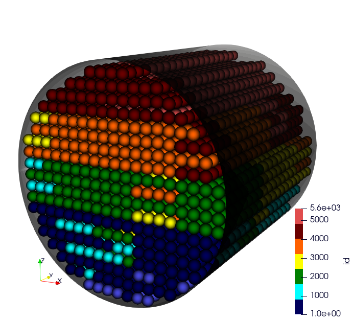
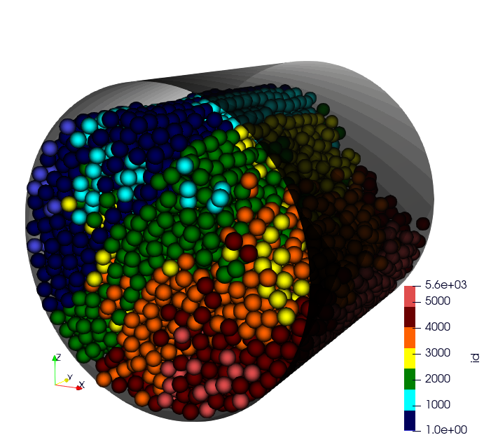
3.1.1. Example 1: Rotating drum
A DEM simulation of a set of spheres in a periodic rotating drum. Through this simulation, we can observe how particles interact, collide, and move in response to the drum’s motion. This provides insights into phenomena like particle segregation, convection currents, and mixing patterns, contributing to improved understanding of granular material behavior in rotational scenarios. A second scenario without periodic conditions is available, with two rigid surfaces fixed to the end of the drum.
Input files:
First test case:
example/spheres/rotating-drum/rotating-drum-periodic.msp5,520 spheres
20,000 timesteps
15.4 seconds on 8 cores (OpenMP)
Second test case:
example/spheres/rotating-drum/rotating-no-periodic.msp27,000 particles
20,000 timesteps
1 minute and 13 seconds on 8 cores (OpenMP)
Third test case:
example/spheres/rotating-drum/rotating-periodic-cohesion.msp1,200 particles
30,000 timesteps
8 seconds on 12 cores (OpenMP)
Rotating Drum |
|
|---|---|
Start |
End |
|
|
|
|
|
|
3.1.2. Example 2: Rigid surface
A DEM simulation involving spherical particles falling onto a rigid surface offers a virtual exploration of particle dynamics in a gravity-driven scenario. This simulation captures the behavior of individual spherical particles as they fall and interact with a solid surface below.
Input file:
example/spheres/rigid-surface/rigid_surface.msp7,360 particles
10,000 timesteps
6.6 seconds on 8 cores
Rigid Surface |
|
|---|---|
Start |
End |
|
|
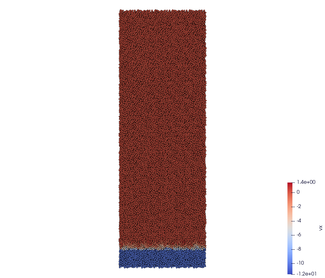
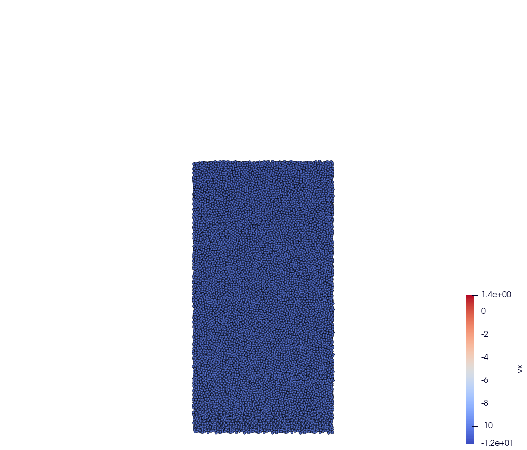
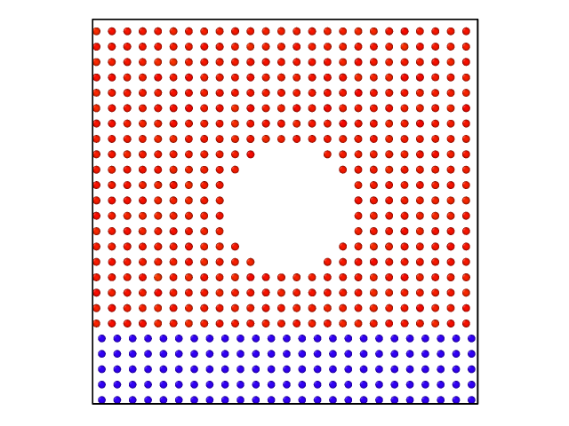
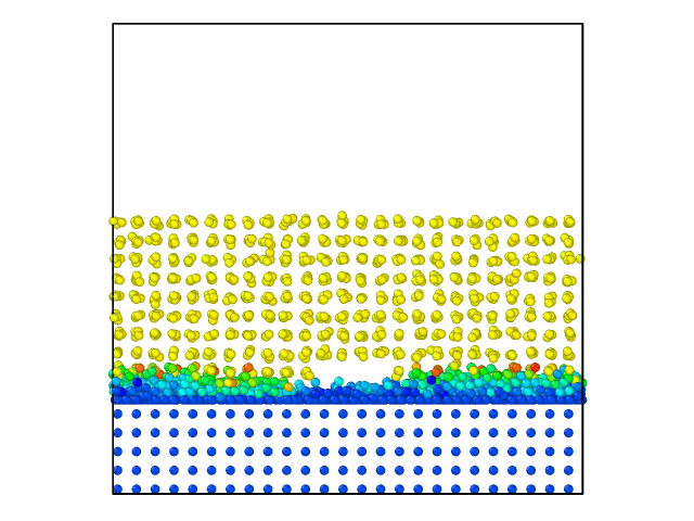
3.1.3. Example 3: Impose Velocity
In this DEM simulation, a scenario is simulated where a group of particles with imposed velocity occupies a defined area. As other particles fall into this region, they interact with the moving particles, impacting their trajectories. The simulation provides insights into how moving driver particles influence the behavior of surrounding particles. Example: impose_velocity_hole, credit: lafourcadp.
Input files:
The first test case:
example/spheres/impose_velocity/impose_velocity_full.msp55,200 particles
10,000 timesteps
1 minute and 40 seconds on 8 cores (OpenMP)
The second test case:
example/spheres/impose_velocity/impose_velocity_hole.msp2,865 particles
2,000 timesteps
1.3 seconds on 8 cores (OpenMP)
Impose Velocity |
|
|---|---|
Start |
End |
|
|
|
|
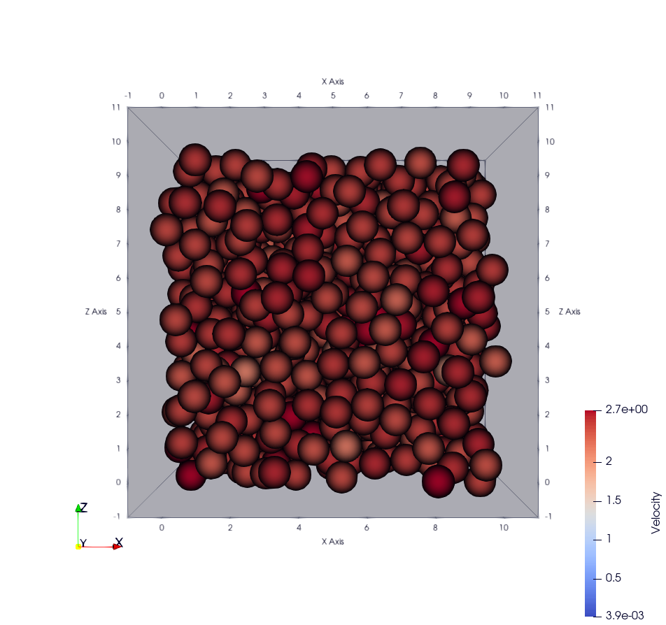
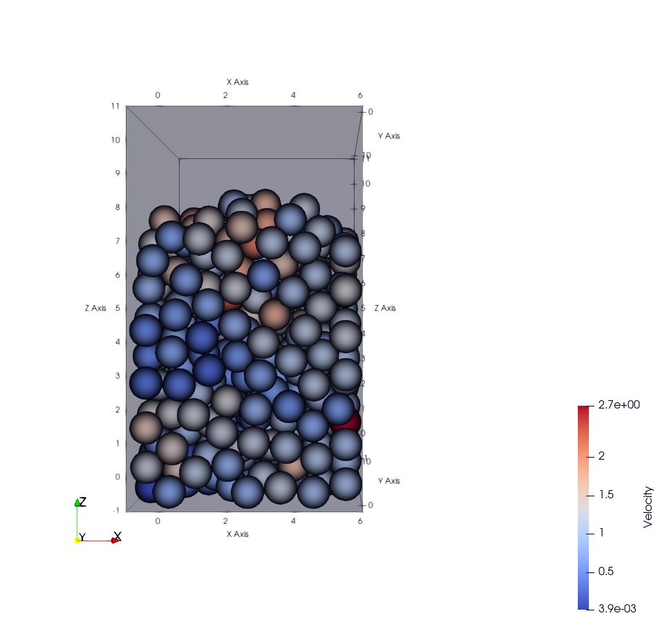
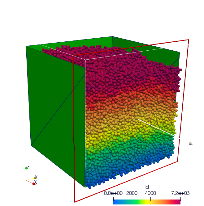
3.1.4. Example 4: Movable wall
In this DEM simulation, a cluster of spherical particles is compacted against a rigid surface. A piston is introduced to apply a steadily increasing stress that linearly evolves over time. This simulation captures the dynamics as the piston’s force gradually grows. As the piston imparts its stress, the particle block undergoes deformation and stress propagation.
Input file:
example/spheres/movable-wall/movable_wall.msp736 particles
30,000 timesteps
4.1 seconds
Movable Wall |
|
|---|---|
Start |
End |
|
|
3.1.5. Example 5: Using a RShape Driver (STL)
In this DEM simulation, a cluster of spherical particles falls onto an .stl mesh and into a box. This case study highlights the use of meshes containing numerous facets and allows adding all geometries coming from CAD or graphic design.
Input file:
example/spheres/mesh-stl/mesh_stl.msp5,000 particles
20,000 timesteps
36.4 seconds on 8 cores (OpenMP)
RShape Driver |
|
|---|---|
Start |
End |
|
|
3.1.6. Example 6: Particle Generation With RSA Algorithm
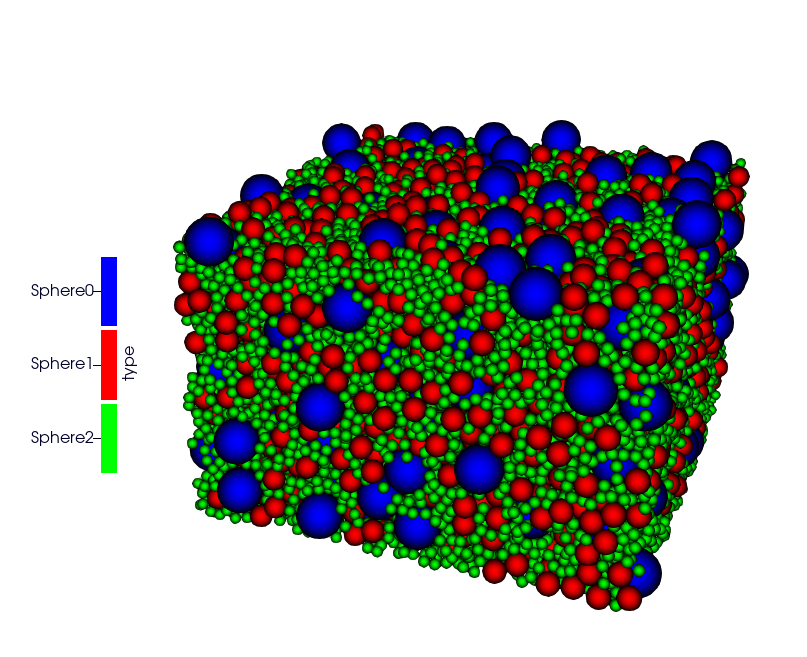
In this DEM simulation, a cluster of 287,642 spherical particles has been generated by the parallelized rsa algorithm [7]. Then, particles fall by gravity in a drum.
Input file: example/spheres/rsa/rsa-full.msp
A second example, available in example/spheres/rsa/rsa_vol_frac.msp, demonstrates how to define different volume fractions for particles of varying sizes.
Note
rsa is an optional package, please see installation guidelines to add it.
RSA |
|
|---|---|
Start |
End |
|
|
|
|
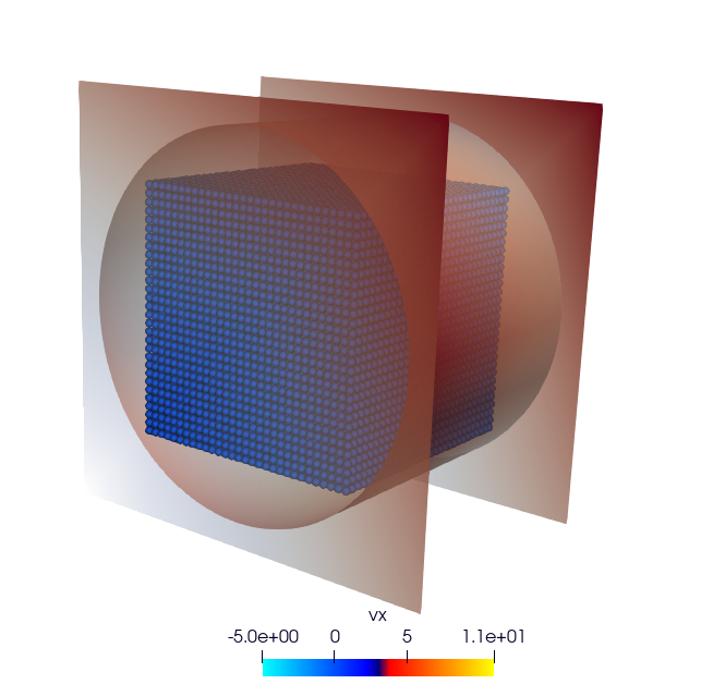
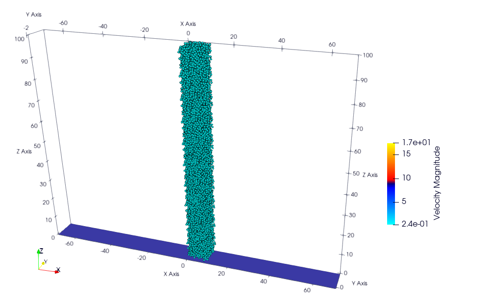
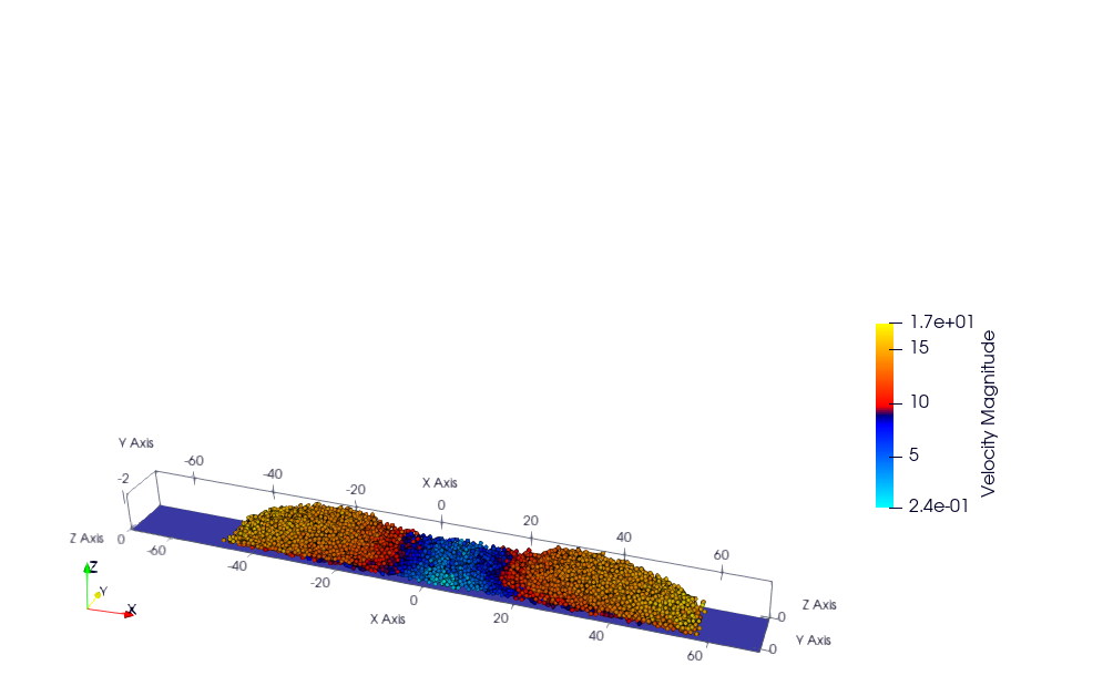
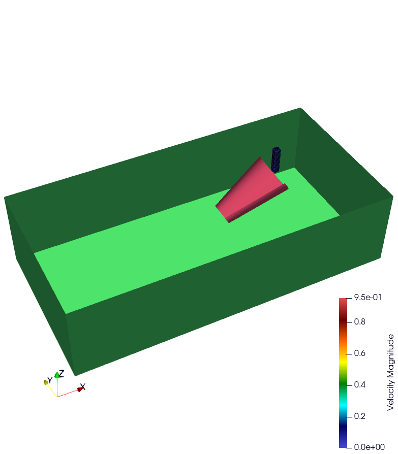
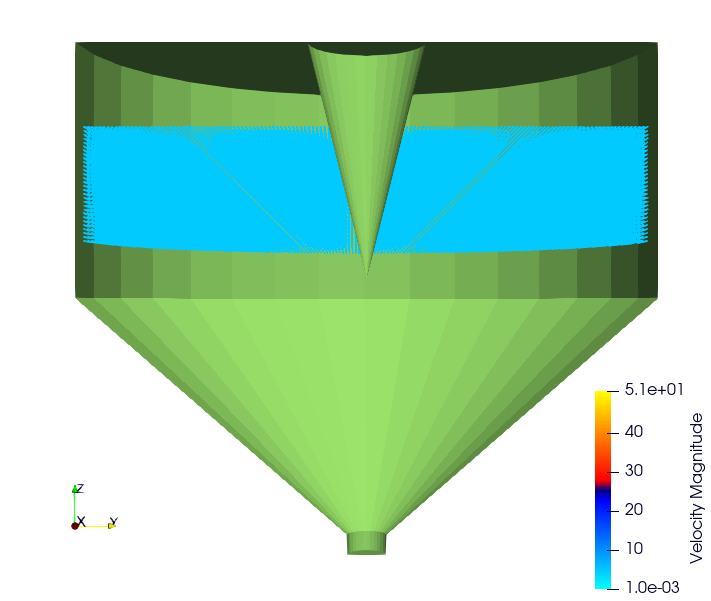
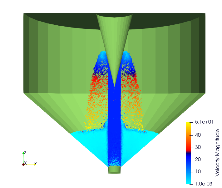
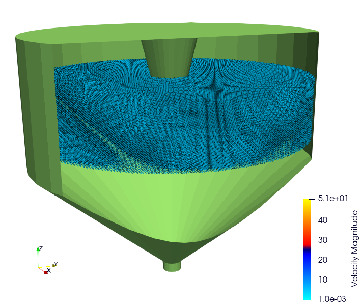
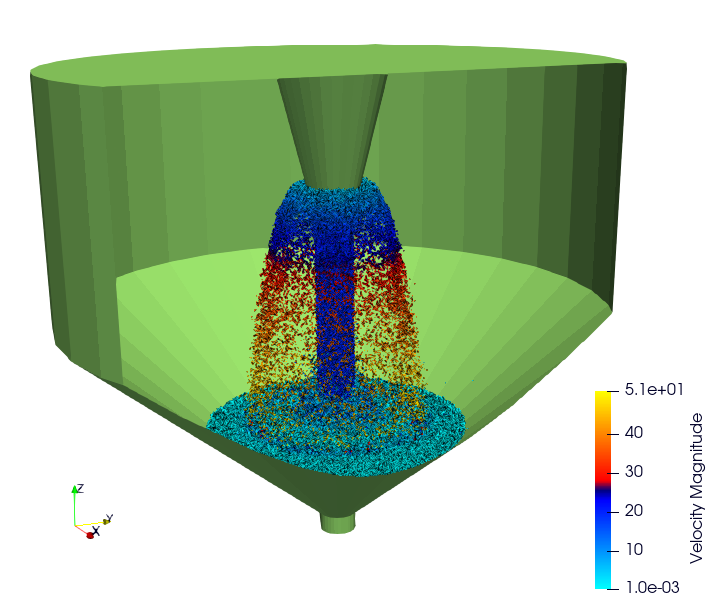
3.1.7. Example 7: Jet
This example demonstrates the application of a velocity field to spheres based on a Cartesian grid projection. Although it does not represent a physical scenario, a geyser-like effect has been simulated using a cylindrical shape, directing the particle velocities towards a specified speed. Future developments will involve applying non-uniform velocity fields to simulate more complex fluid configurations. Input files are available here: example/spheres/jet/step1.msp and step2.msp but they don’t correspond exactly to the pictures (fewer particles).
Geyser Simulation |
|
|---|---|
Start |
End |
|
|
|
|
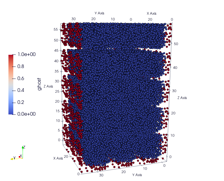
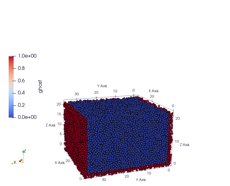
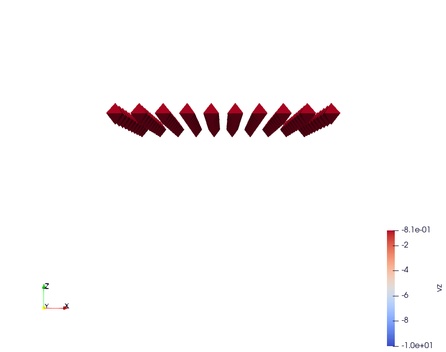
3.1.8. Example 8: Mirror Boundary Conditions
This example tests the mirror conditions available in exaNBody. Although these conditions are not directly applicable (” not physics “), because all fields are copied identically (without processing/filtering) at each time step in the ghost cells (e.g. velocity, moments), except for positions (axial symmetry). This example highlights this functionality and could potentially be coupled with other operators to develop new boundary conditions (e.g. resetting velocities to 0 to model a rigid surface). This example involves dropping 33,120 spheres, adding mirror boundary conditions in all directions, and letting them fall by gravity.
Input file:
example/spheres/mirror/mirror.msp.33,120 particles
5,000 timesteps
21.8 seconds on 8 cores (OpenMP)
Mirror Simulation |
|
|---|---|
Start |
End |
|
|
3.2. Examples Using Polyhedra
All examples with polyhedra can be found in the directory: example/polyhedra/.
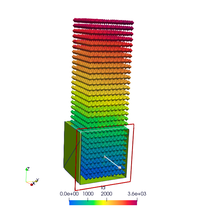
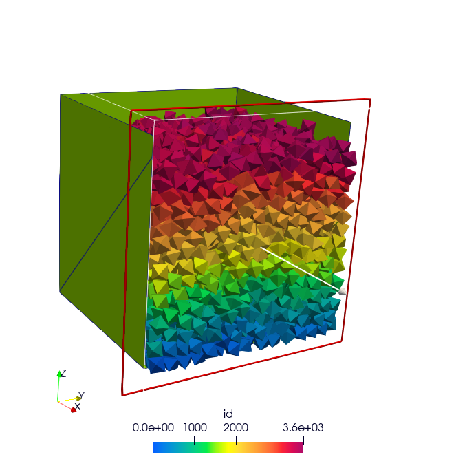
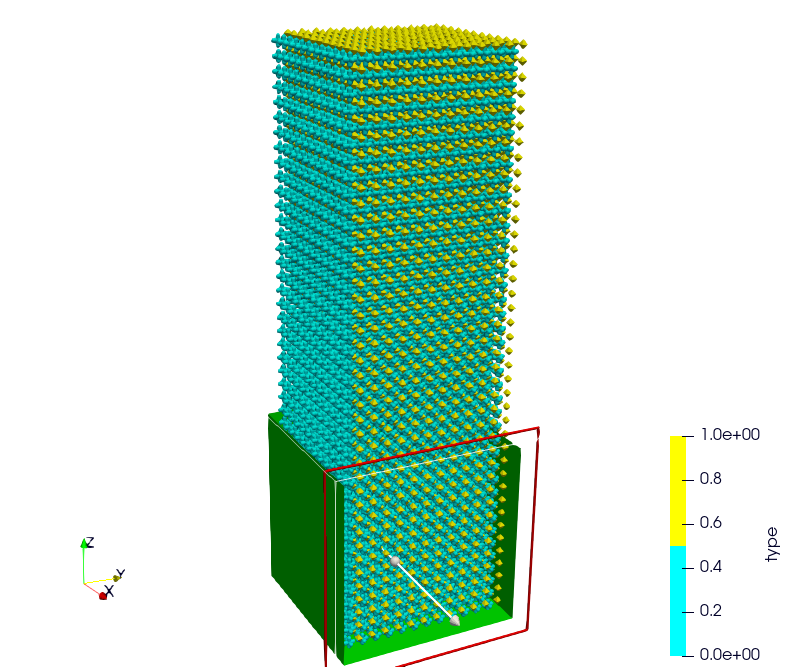
3.2.1. Example 1: Polyhedra Generation Frequency
In this example, we simulate the generation of 100 new polyhedra at every 45000 time steps, representing their descent into a void environment. The primary objective is to illustrate the process of generating a lattice of polyhedra within a confined area. Additionally, we demonstrate the application of a series of operators to initialize various fields associated with the newly generated polyhedra. This example serves as a practical guide for setting up and executing simulations involving dynamic polyhedra generation and manipulation within defined spatial boundaries.
Input file:
example/polyhedra/generator/generator.msp100 then 200 and 300 Octahedra
10,000 timesteps
9.7 seconds on 8 cores (OpenMP)
Polyhedra Generation Frequency |
|
|---|---|
Start |
End |
|
|
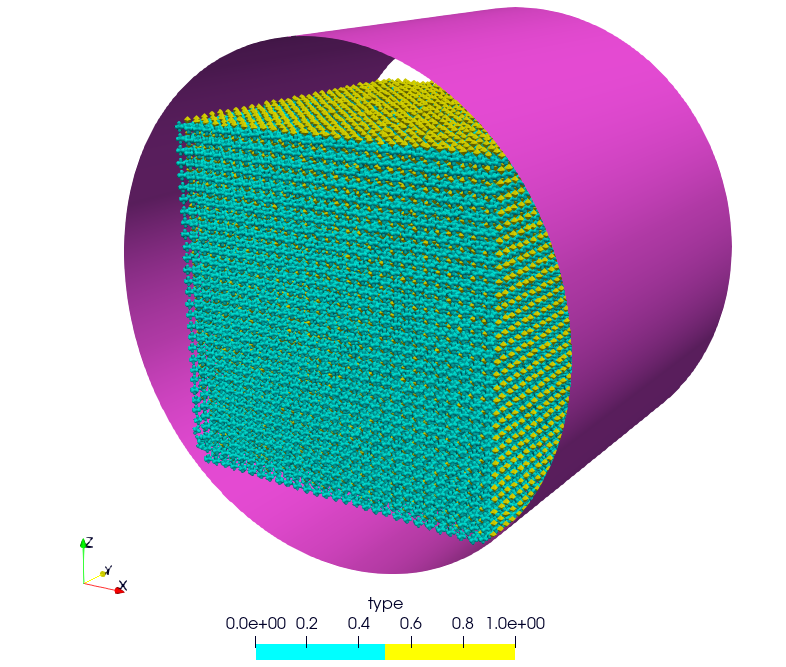
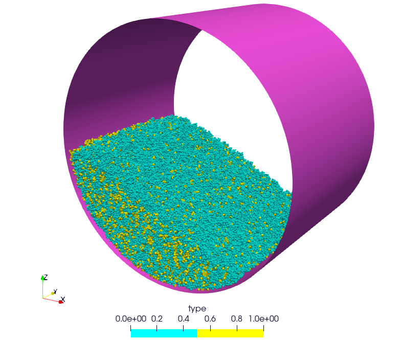
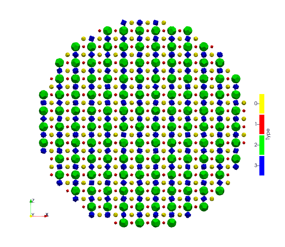
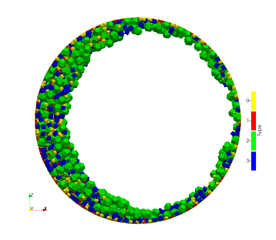
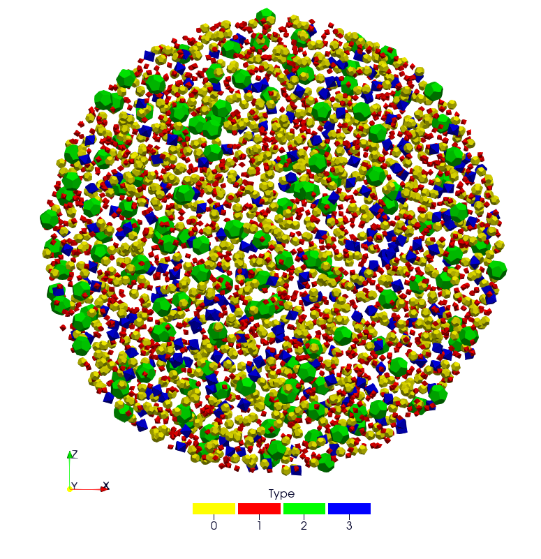
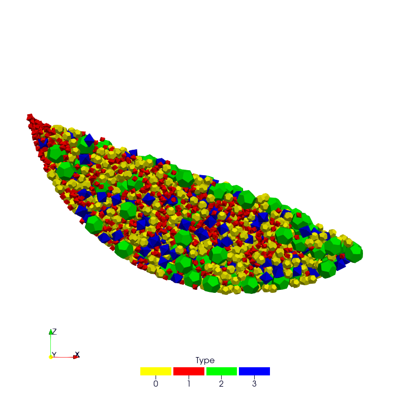
3.2.2. Example 2: Octahedra in a Rotating Drum
In this DEM simulation, we observe the dynamics of 125 octahedra as they descend into a rotating drum. The second test case contains 27,000 octahedra (yellow) and 27,000 hexapods (blue).
Input files:
The first example:
example/polyhedra/rotating_drum/rotating-drum-mini.msp125 Octahedra
10,000 timesteps
1 second on 8 cores (OpenMP)
The second example:
example/polyhedra/rotating_drum/rotating-drum-mixte.msp27,000 Octahedra and 27,000 Hexapods
100,000 timesteps
41 minutes and 36 seconds on 8 cores (OpenMP)
6 minutes and 31 seconds on a100 (100,000 timesteps) with rcut_inc = 0.4
11 minutes and 24 seconds on a100 (200,000 timesteps) with rcut_inc = 0.4 (The stage where the particles fall is costly, as the particles are quickly moved from one cell to another, and the reconstruction of neighbor lists (on the CPU) is also costly.)
The pictures correspond to the simulation after 1,000,000 timesteps
Other example:
example/polyhedra/rotating_drum/rotating-drum.msp5520 Octahedra
150,000 timesteps
2 minutes and 19 seconds on 8 cores (OpenMP)
Other example:
example/polyhedra/rotating_drum/rotating-drum-mixte-mini.msp125 Octahedra and 125 Hexapods
20,000 timesteps
2.5 seconds on 8 cores (OpenMP)
Polyhedra Generation Frequency |
|
|---|---|
Start |
End |
|
|
|
|
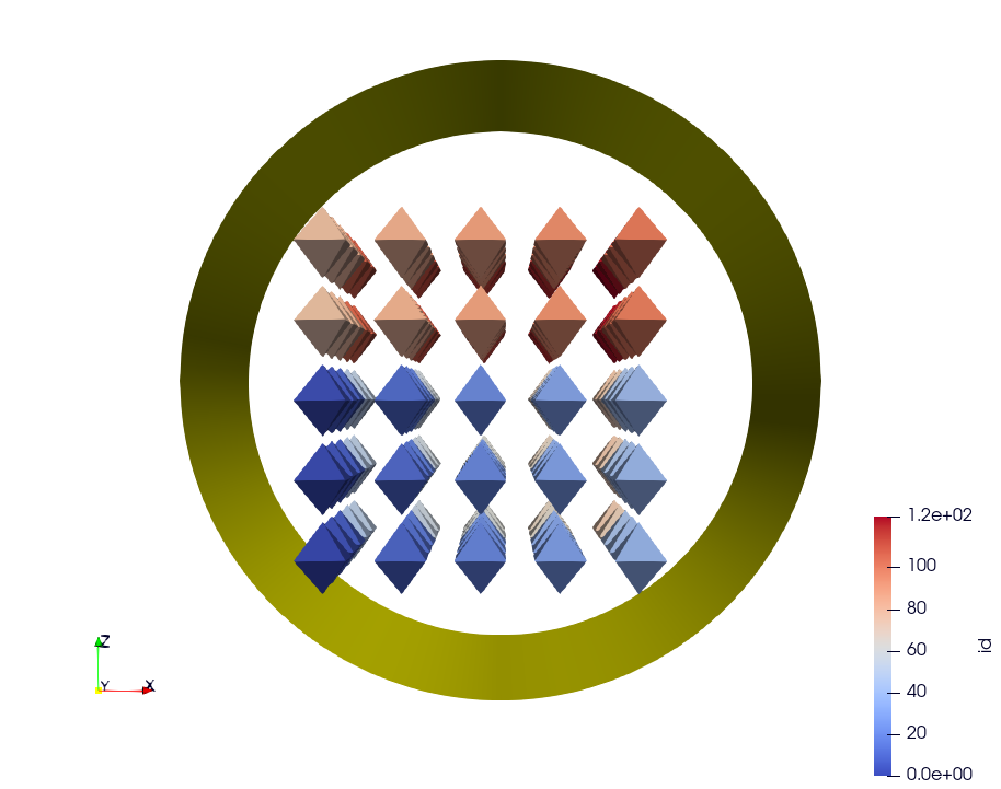
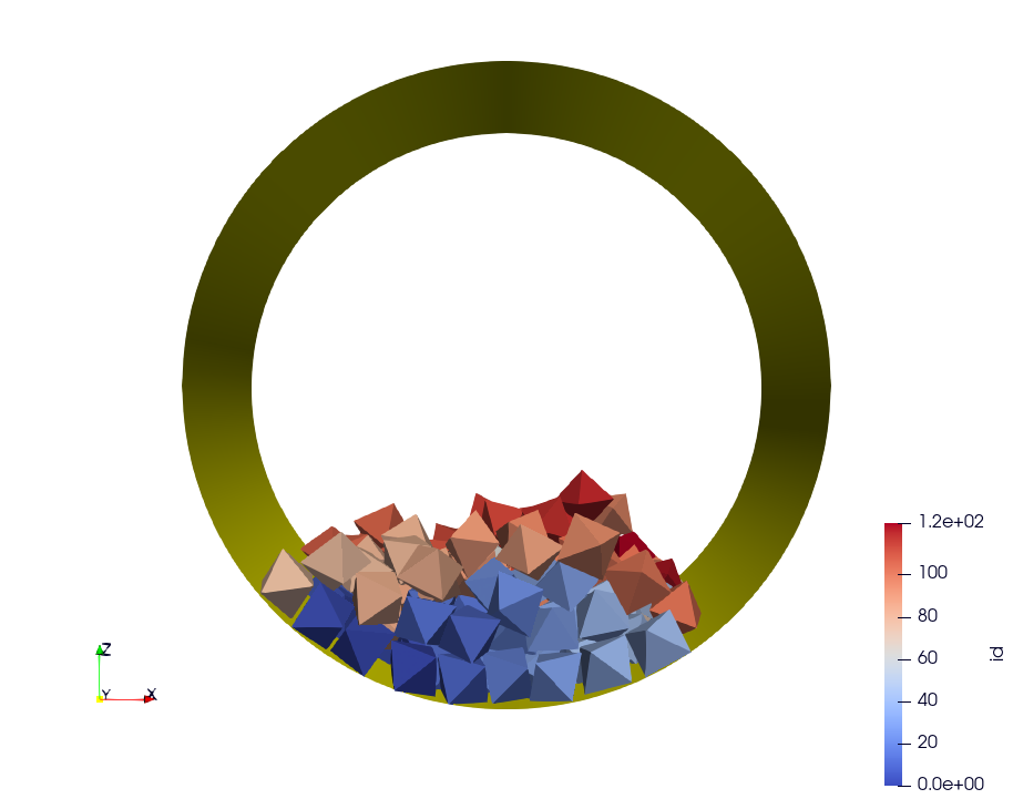
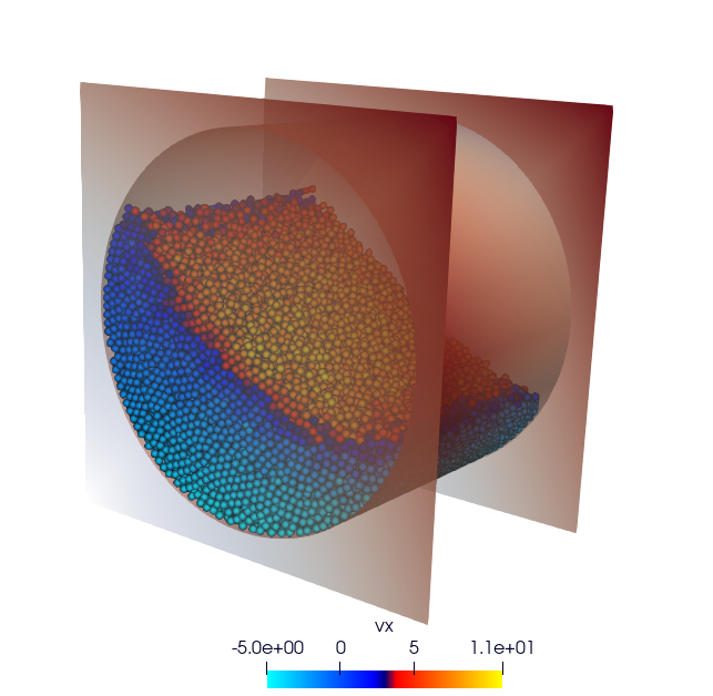
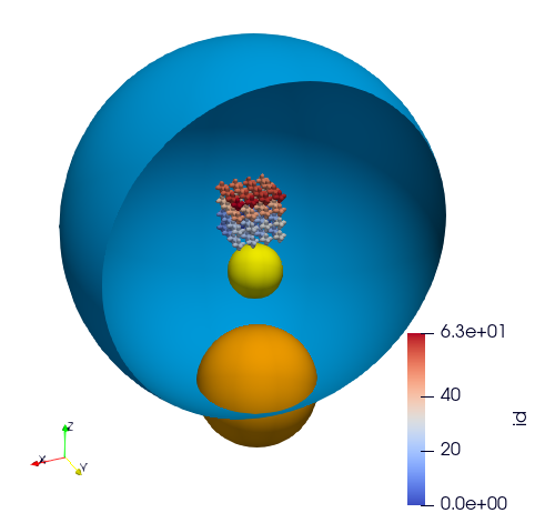
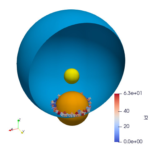
3.2.3. Example 3: Hexapods in a Ball
This DEM simulation example illustrates the gravitational descent of 64 hexapods within a large sphere. The primary environment consists of a spherical enclosure with a radius of 20 units and is centered at (2, 2, 0). As the hexapods descend under gravity within this enclosure, they encounter two additional spherical obstacles. The first obstacle (ball, represented as a small yellow ball with a radius of 3 units and centered at (2,2,-5). The second ball, centered at (2,2,-20) with a radius of 7 units, depicted as a large orange ball, intersects the surface of the primary blue sphere, adding complexity to the obstacle configuration. Through this simulation, exaDEM shows its capability to manage particle interactions with various obstacles (balls). Additionally, it showcases the versatility of drivers within the code, which can be employed to define both simulation boundary conditions and obstacles.
Input file:
example/polyhedra/balls/balls.msp64 Hexapods
150,000 timesteps
14.3 seconds on 8 cores (OpenMP)
Other example:
example/polyhedra/balls/balls.msp64 Hexapods
25,000 timesteps
2.7 seconds on 8 cores (OpenMP)
Hexapods in Ball |
|
|---|---|
Start |
End |
|
|
3.2.4. Example 4: Polyhedra With a RShape Driver (Box)
This simulation example illustrates the use of STL files with polyhedra. In this simulation, we drop a set of polyhedra (hexapods, octahedra, or both) by gravity into an open box to fill it completely.
Input files:
First example:
example/polyhedra/stl_mesh/stl_mesh_box_hexapod.msp7,344 Hexapods
50,000 timesteps
2 minutes and 19 seconds on 8 cores (OpenMP)
Second example:
example/polyhedra/stl_mesh/stl_mesh_box_octahedron.msp2,430 Octahedra
50,000 timesteps
1 minute and 6 seconds on 8 cores (OpenMP)
Third example:
example/polyhedra/stl_mesh/stl_mesh_box_mixte.msp5760 Octahedra and 5760 Hexapods
100,000 timesteps
8 minutes and 36 seconds on 8 cores (OpenMP)
2 minutes and 34 seconds on a GPU a100 (rcut_inc = 0.2, cell_size = 6, and grid_dims = [3,3,10])
Note
These examples have minimal test cases (_mini.msp).
Polyhedra With a RShape Driver |
|
|---|---|
Start |
End |
|
|
|
|
|
|
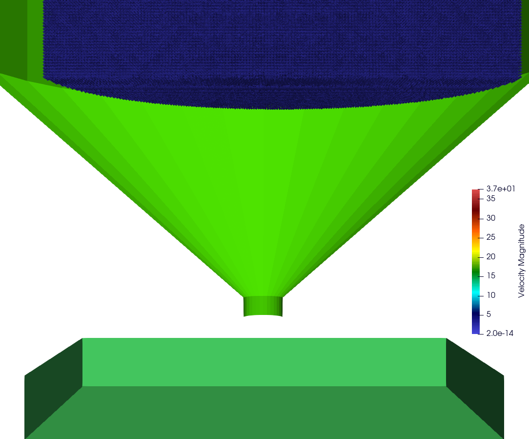
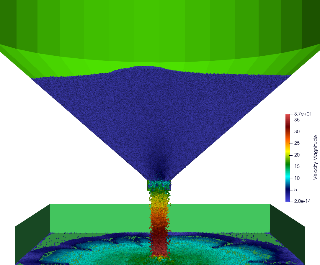
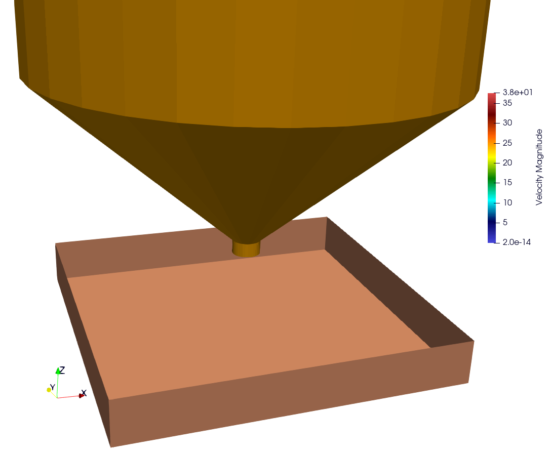
3.2.5. Example 5: Funnel
This simulation example illustrates the gravitational drop of a set of 1.3 million hexapods into a funnel. The funnel is represented using a mesh of faces (RShape Driver).
Input file:
example/polyhedra/funnel/funnel.msp
Note
This example is designed to run on a supercomputer or recent GPUs, so don’t run it on a laptop.
Polyhedra With a Funnel |
|
|---|---|
Start |
End |
|
|
|
|

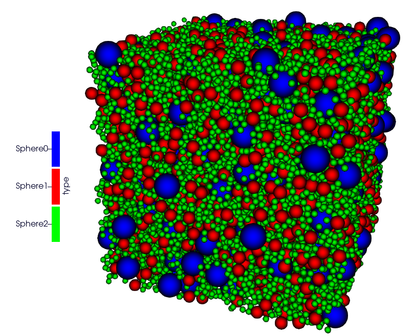
3.2.6. Example 6: Rescale shape
In this simulation, two shapes are selected: PolyR and Octahedron. Each shape is then duplicated with its size doubled, resulting in PolyRSize2 and OctahedronSize2. The setup is a rotating drum, where particles are generated using two different methods: FCC and RSA. The simulation runs for 1,000,000 time steps with a time step size of dt = 5e-5.
Input files:
FCC:
example/polyhedra/rescale_shape/scale_2_shapes_fcc.msp2,144 polyhedra or 536 polyhedra of each type
1,000,000 timesteps
1 hour and 23 minutes on 12 cores (OpenMP)
RSA:
example/polyhedra/rescale_shape/scale_2_shapes_rsa.msp3,698 polyhedra, the volume fraction used for every type is 0.055
1,000,000 timesteps
38 minutes on 12 cores (OpenMP)
Rescale Shapes |
|
|---|---|
Start |
End |
|
|
|
|
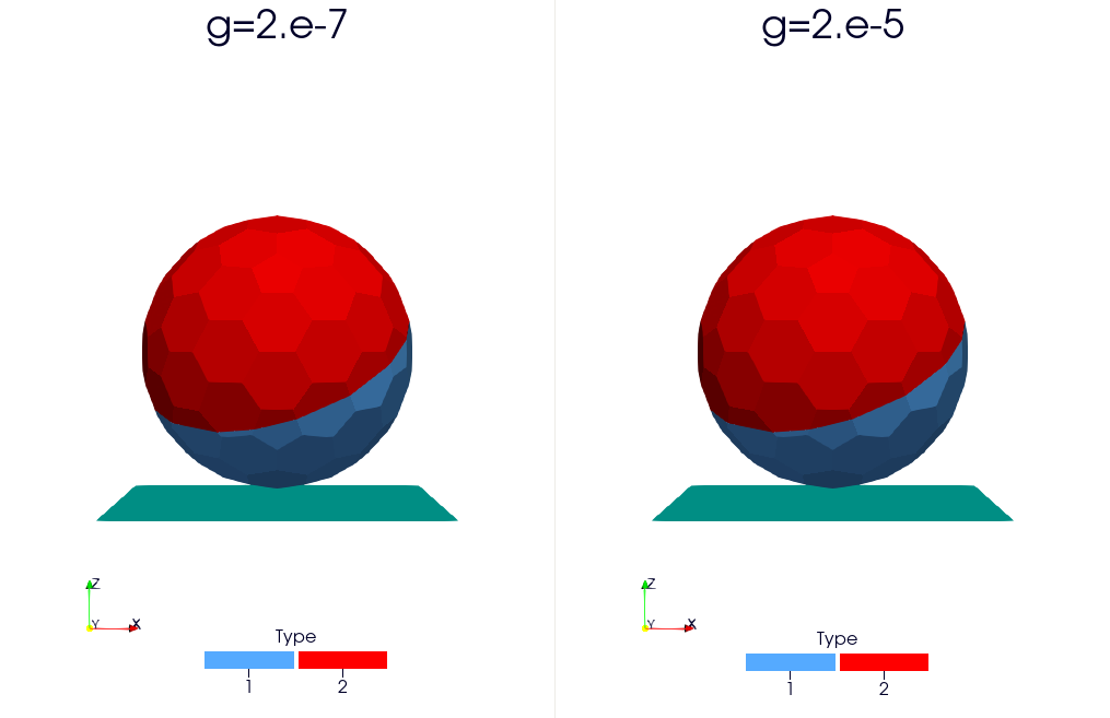
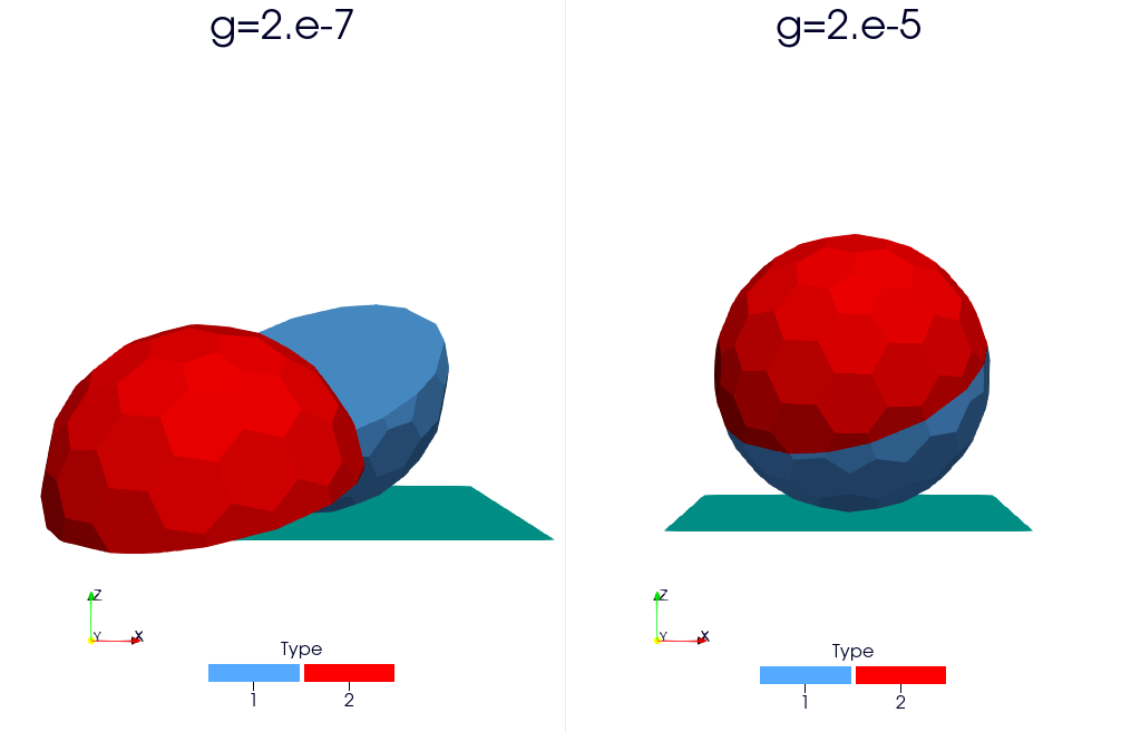
3.2.7. Example 7: Fragmentation with two fragments
This simulation demonstrates the fragmentation capability. The test case considers a grain composed of two fragments that is rapidly projected onto a rigid surface. Two configurations are compared. In the first one, the grain remains intact because the breakage criterion, governed by the parameter g, is not reached. In the second configuration, a lower value of g leads to the failure of the interface between the two fragments, resulting in fragmentation.
Input files:
With Crackling:
example/polyhedra/fragmentation/two_fragments_break.msp2 fragments
1,800,000 timesteps
84 seconds on 1 core
No Crackling:
example/polyhedra/fragmentation/two_fragments_unbreak.msp2 fragments
1,800,000 timesteps
68 seconds on 1 core
Grain composed of two fragments |
|
|---|---|
Start |
End |
|
|
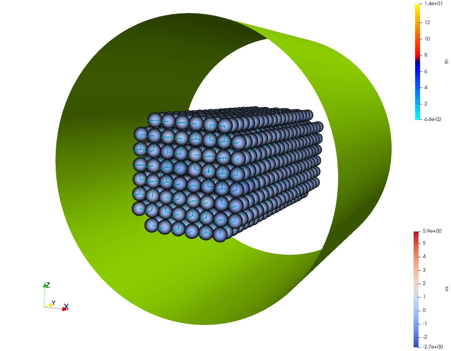
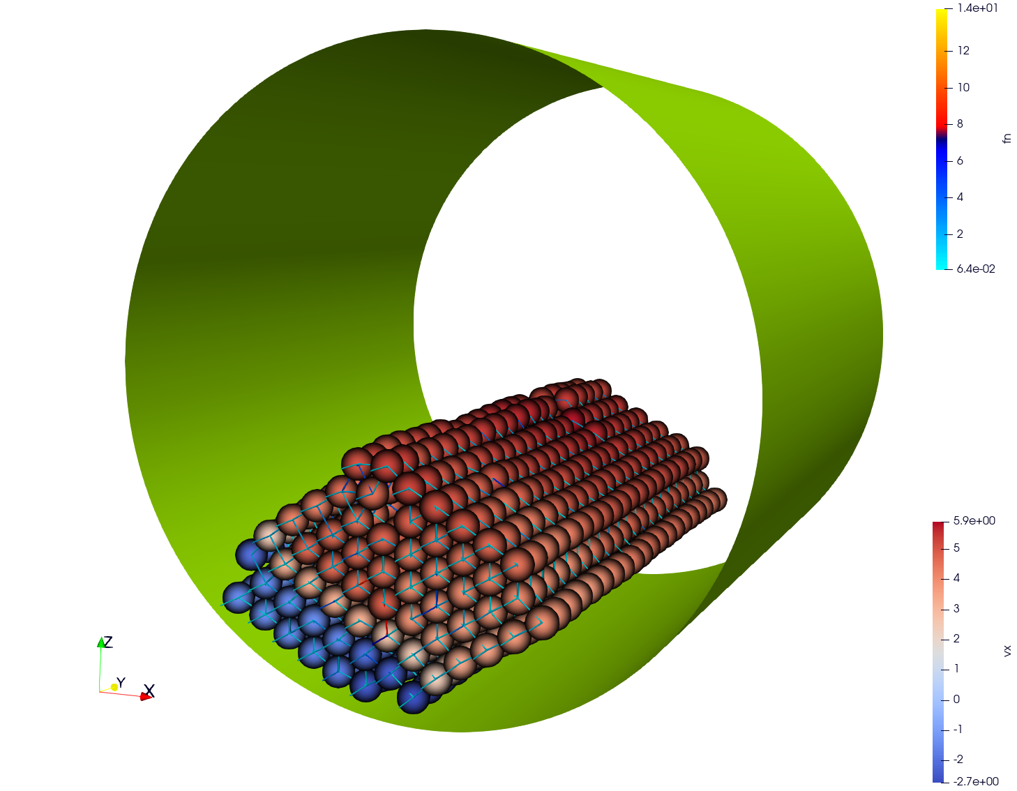
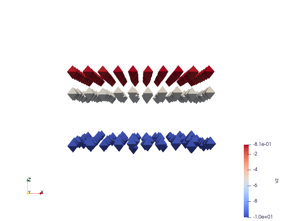
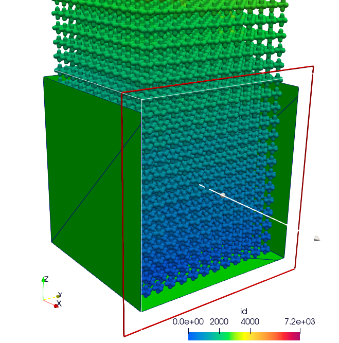
3.2.8. Example 8: Impact of a Sphere
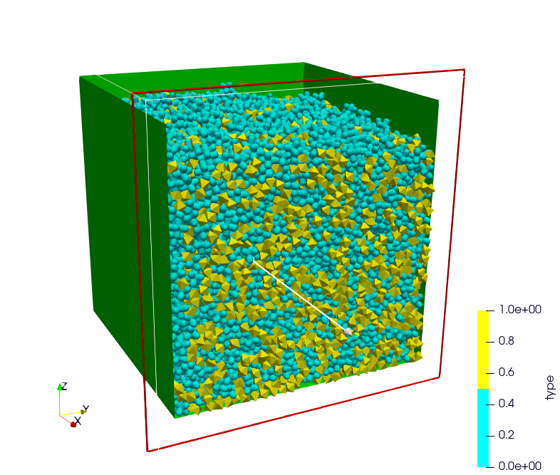
This simulation reproduces the impact of a high-speed projectile on a wall composed of cubic particles. These particles are linked by cohesive interactions (springs) between the vertices of their faces. The wall is placed on a surface with a high friction coefficient to prevent it from shifting. This simulation also incorporates a periodic boundary condition along the direction of the wall.
Input files:
exaDEM/example/polyhedra/basic_shape/impact_with_frag.msp1,601 particles
300,000 timesteps
445 seconds on 12 cores
Impact |
|
|---|---|
Start |
End |
|
|

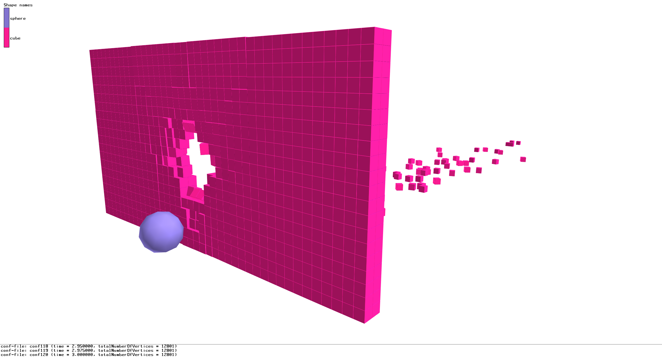
Front view:
Back view:
3.3. Show-cases
3.3.1. On a laptop or single node
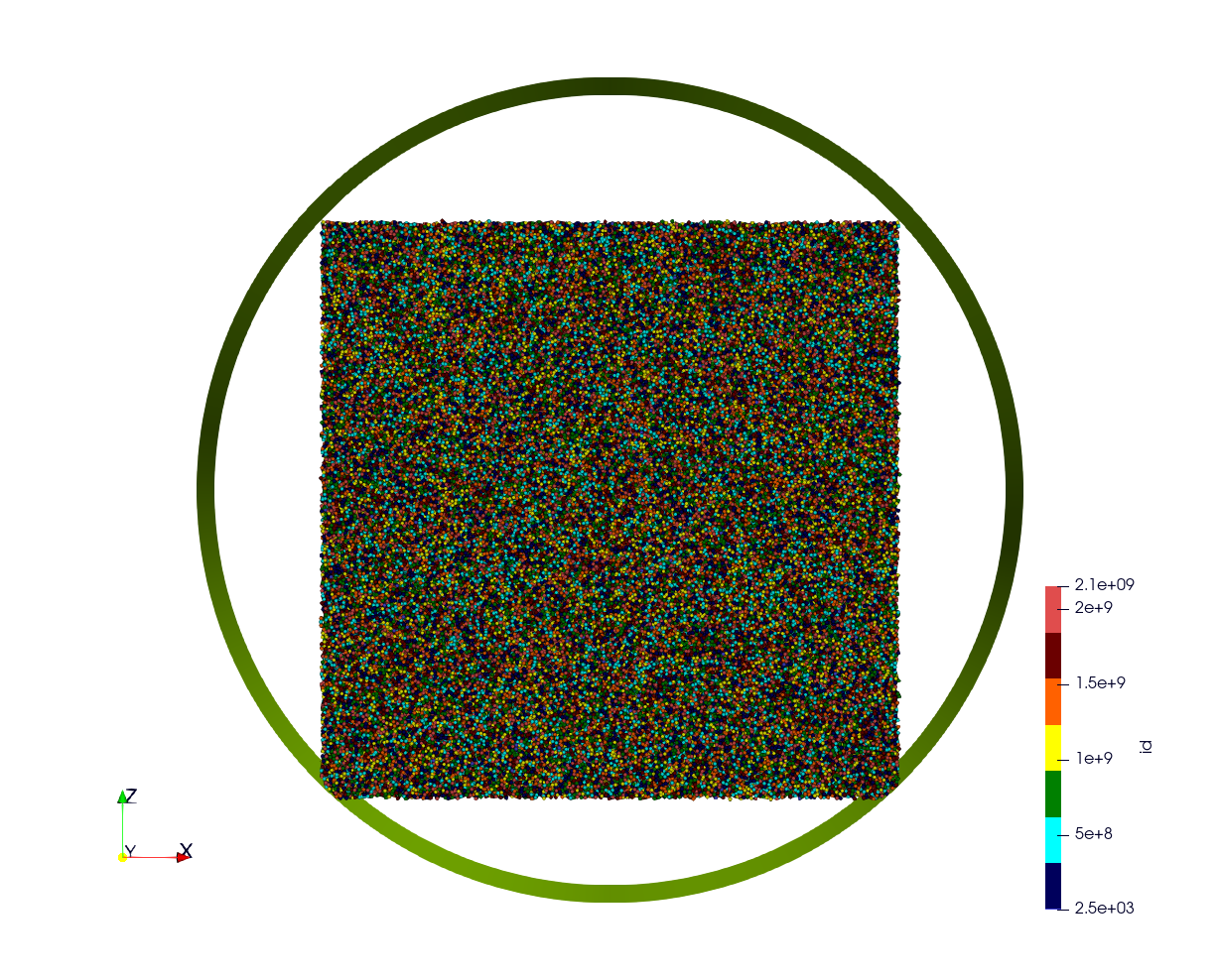
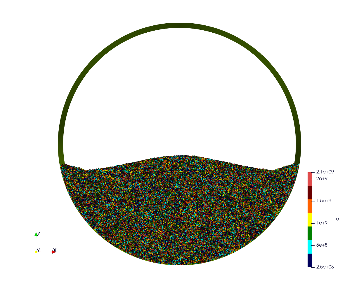
3.3.1.1. Rotating drum simulation
Simulation of 48,000 spheres on a rotating drum after reading an .stl file. This simulation takes around one hour and 10 minutes on a laptop with 12 cores with OpenMP. The input files are available here: example/spheres/cylinder_stl/cylinder_stl.msp
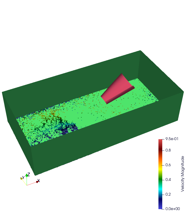
Simulation of 140,000 spheres falling into a cell. A blade is then activated with rotational and translational motion. This simulation takes around 4-5 days on a single node of 32 cores. A tutorial is available with polyhedra in the tutorial section.
TODO: Add input files
3.3.2. On a supercomputer
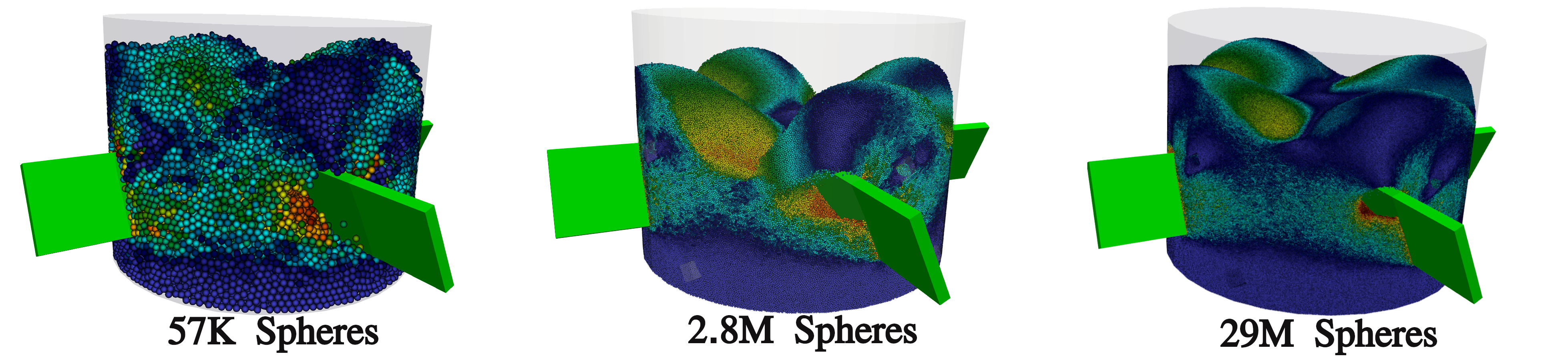
3.3.2.1. Mixer simulation
Simulation of a mixer into which spherical particles are falling. The simulation consists of rotating a propeller at 0.25 rad/s while using progressively smaller grains. This simulation is based on an example provided in the chronoDEM::gpu code and described in the following paper: “Chrono::GPU: An open-source simulation package for granular dynamics using the discrete element method” [6].
To accelerate simulation time, the time step was increased to 1×10⁻³, and the contact law parameters were adjusted accordingly.
The input files for the different scenarios are available in: exaDEM/example/spheres/mixer
mixer_57k_sph.msp
mixer_3M_sph.msp
mixer_29M_sph.msp
Below is an image showing the different scenarios based on the number of particles: