4.8. Post Processings
In this section, we will describe the operators related to the usage of polyhedra or spheres.
4.8.1. Paraview For Polyhedra
- In exaDEM, there are two ways to display polyhedra with Paraview:
The first is to directly display the vertices of the polyhedra and the surfaces in parallel VTP (PolyData). However, no fields associated with the polyhedra are available, such as velocity or density.
The second solution is to use the generic Paraview output of exaDEM by adding the orientation field and the homothety field (optional). Then, it’s possible to associate a mesh with each point, such as an octahedron.vtk file generated by read_shape_file, to each point by associating it with a size (field::homothety) and a quaternion (field::orient).
Note
Only the default behavior when the config_polyhedra.msp file is used is the option 2 that offers more possibilities. In addition, it is important to note that paraview does not include the layer of shape->radius size, i.e. faces are displayed according to the vertex centers.
- Option 1: write_paraview_generic
binary_mode [BOOL] : paraview format file, default is true.
compression [STRING] : level of compression, default is “default” for vtkZLibDataCompressor.
filename [STRING]: basename of the parallel paraview output files, default is “output”.
write_ghost [BOOL]: dump ghost particles, default is false.
write_box [BOOL]: write box information in a box.vtp file, default is true.
write_external_box [BOOL]: write external box (ghost area), default is false.
This operator is based on this function: ParaviewWriteTools::write_particles.
YAML example:
write_paraview_generic:
  binary: false
  write_ghost: false
  fields: ["vx","vy","vz","id","orient"]
How to use it with Paraview:
Firstly, we need to load our reference mesh (Octahedron.vtk) in our case.
Secondly, load your particle file into the Paraview folder (default name in exaDEM for the paraview_generic operator).
Thirdly, choose the 3D Glyphs representation and the coloring.
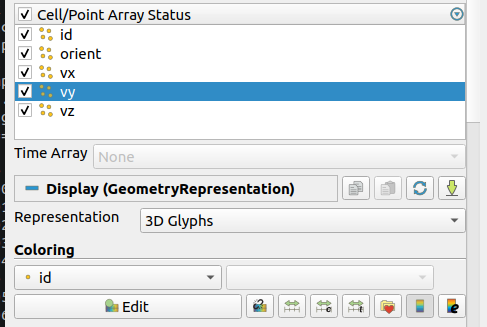
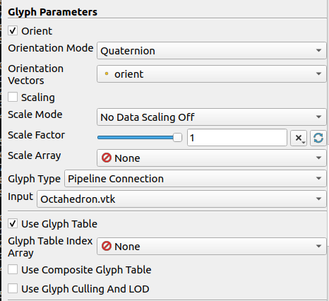
Fourthly, in the Glyph Parameters section, choose “Orient” with the orientation mode “Quaternion” and as orientation vectors: “orient”. To change the size, you can check Scaling and add the Scale Array you wish. Finally, in the Glyph Type dropdown menu, select “Pipeline Connection” and in Input, choose “Octahedron.vtk”.
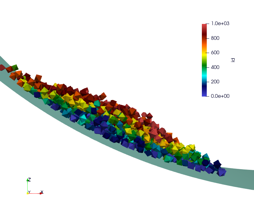
Result for a simulation of 1000 Octahedra falling in a cylinder colored by their ID:
- Option 2: write_paraview_polyhedra
filename : Name of paraview file, there is no default name. Note that in ExaDEM, filename is defined in the default execution stream.
mpi_rank : Add a field containing the mpi rank. [optional]
YAML example:
particle_write_paraview_generic:
  - write_paraview_polyhedra:
     mpi_rank: true
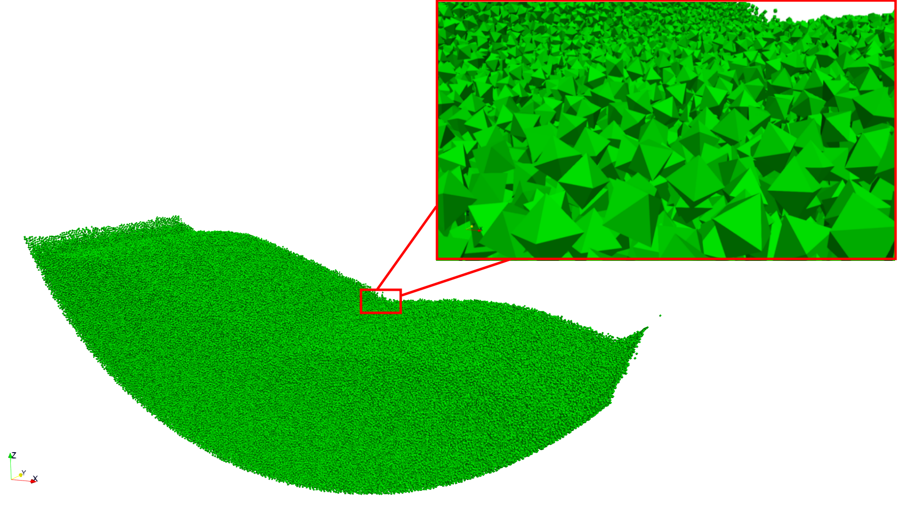
Example with 850,000 octahedra:
Note
This operator is rather limited in terms of visualization, so we now advise you to use option 1, which offers more possibilities (field display) and less memory-intensive files.
4.8.2. Paraview With OBB
This operator allows you to display OBBs around polyhedra in paraview. These files are stored in different files from those used to store polyhedron information. By default, these files are available in the directory ExaDEMOutputDir/ParaviewOutputFiles/ under the format obb_%010d.pvtp. The fields associated with OBBs are the polyhedron ID and type.
- write_paraview_obb_particle:
basedir : Name of the directory where paraview files will be written
basename : Name of paraview file, there is no default name. Default is “obb”.
timestep : Current simulation time is defined.
Note
This operator is called after write_paraview_generic and is triggered by simulation_paraview_frequency called into the global operator.
Warning
This operator doesn’t work for simulations with spheres.
YAML example:
- write_paraview_obb_particle
Output example:
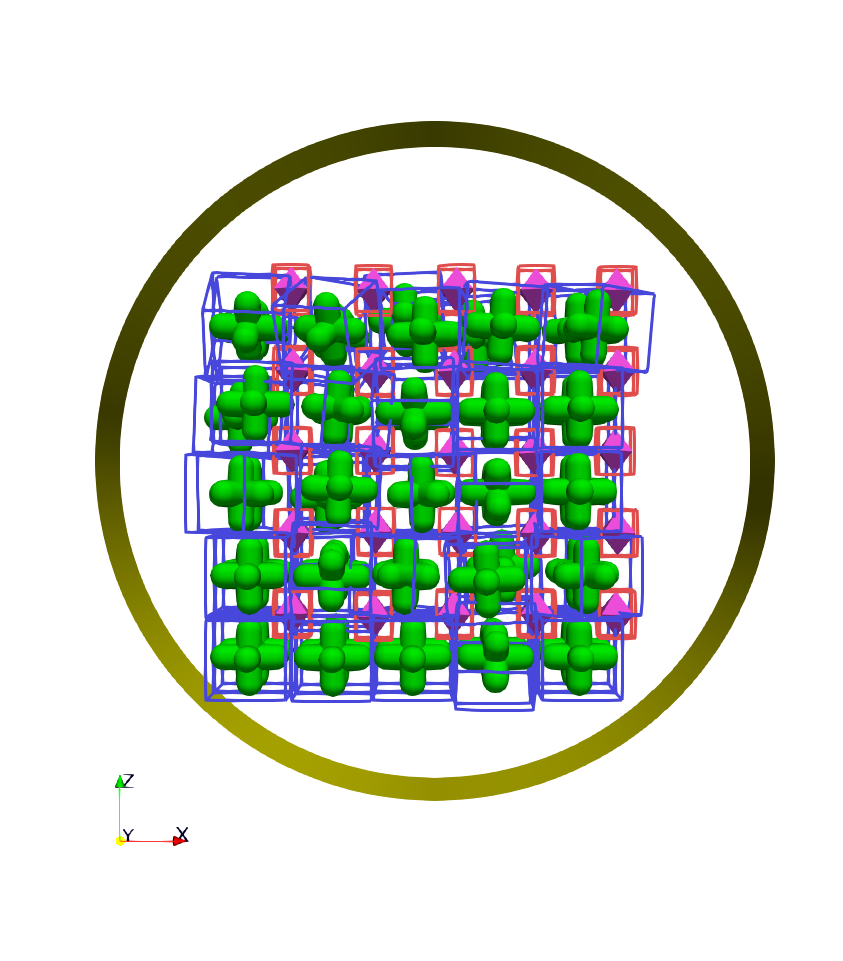
4.8.3. Contact Network
This operator is used to visualize the contact network between polyhedra using ParaView. For each active contact/interaction, we assign the value of the normal force calculated in Contact’s law. You can enable this option, which will be automatically triggered at the same time as the other paraview files, with the option enable_contact_network: true in global. See examples: “Polyhedra/Example 2: Octahedra in a Rotating Drum” and “Spheres/Example 1: Rotating drum”.
- dump_contact_network:
filename : Name of the paraview file, there is no default name.
timestep : Current simulation time is defined.
YAML example:
- timestep_paraview_file: "ParaviewOutputFiles/contact_network_%010d"
- dump_contact_network
global:
  enable_contact_network: true
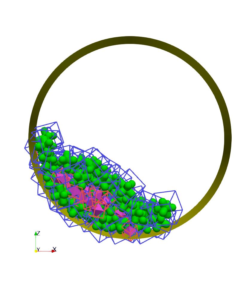
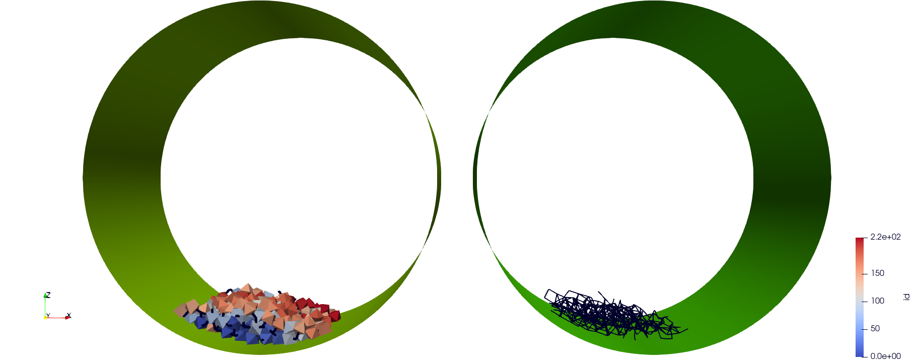
Here is an example of 216 polyhedra after a fall into a cylinder, left the simulation and right the contact network:
Comments / Extensions:
This operator can be modified to display more values per contact. To achieve this, you need to change the type of StorageType in the NetworkFunctor structure. Then, you’ll need to populate this function in the operator () (exaDEM::Interaction* I, const size_t offset, const size_t size). Finally, you’ll need to add a field in write_pvtp and include this field in write_vtp.
Currently, this operator doesn’t take particularly long to execute and isn’t called frequently. However, it doesn’t benefit from any shared-memory parallelization (OpenMP) because the network storage is implemented using a std::map.
4.8.4. Project Field Quantities onto Cartesian Grid
This operator projects the sum of one or several field values onto a Cartesian grid corresponding to the grid defined by the cells of the DEM mesh. It is then possible to use the write_grid_vtklegacy operator to generate a Paraview output.
Operator description:
Name:
quantities_cell_projectionParameters:
fields [list of strings]: List of regular expressions to select fields to project. Example: fields: [vx, ay, stress].
grid_subdiv [double]: Number of subdivisions applied to each grid cell. Default is 1, i.e no subdivision.
splat_size [int >= 1]: Smoothing factor controlling the spatial influence of each projected value. Default is 1.0.
to use this operator, the simplest way is to define the analysis frequency (all) in the global operator (simulation_analyses_frequency) and add the quantities_cell_projection operator to the operator analyses, as in the following example (see example/polyhedron/analysis/particle_cell_projection.msp:
YAML example: available here example/polyhedron/analysis/particle_cell_projection.msp
global:
  simulation_analyses_frequency: 1000

analyses:
  - timestep_paraview_file: "ParaviewOutputFiles/quantities_%010d.vtk"
  - message: { mesg: "Write " , endl: false }
  - print_dump_file:
      rebind: { mesg: filename }
      body:
      - message: { endl: true }
  - resize_grid_cell_values
  - quantities_cell_projection:
     splat_size: 0.99
     grid_subdiv: 2
     fields: [count, vnorm, vx, vy, vz, stress]
  - write_grid_vtklegacy
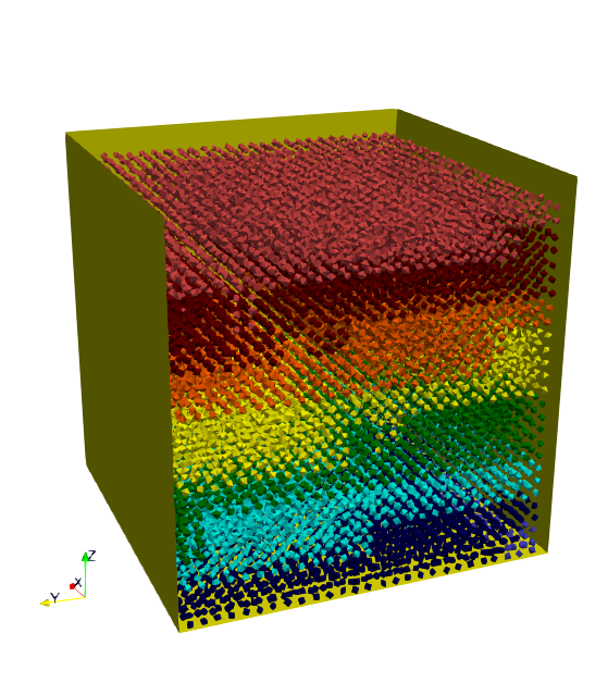
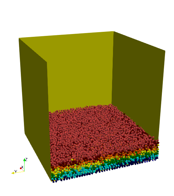
Paraview output:
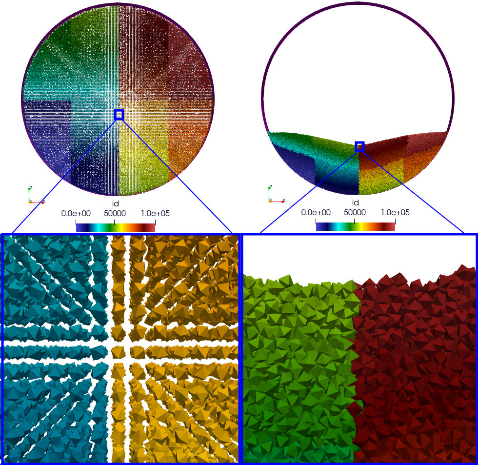
In this figure, we show:
Left: the relative velocity (surface plot),
Middle: a glyph representation of the grid using arrows,
Right: a zoomed-in view showing the octahedra.
ExaDEM provides several pre-configured cell projection examples in data/config/config_cell_projection.msp:
all_cell_proj:description: Projects all available fields.
output:
ParaviewOutputFiles/quantities_XXX.vtk
vnorm_cell_proj:description: Projects the sum of particle velocity norms in each cell.
output:
ParaviewOutputFiles/vnorm_XXX.vtk
velocity_cell_proj:description: Projects particle velocity magnitude and components (vx, vy, vz).
output:
ParaviewOutputFiles/velocity_proj_XXX.vtk
stress_cell_proj:description: Projects the stress field.
output:
ParaviewOutputFiles/stress_proj_XXX.vtk
count_cell_proj:description: Counts the number of particles per cell.
output:
ParaviewOutputFiles/count_proj_%010d.vtk
Note
For all of these post-processing operators, the count output is also added to allow computing averages of projected quantities.
These operators don’t use the subgrid option.
YAML example:
Full source code: example/polyhedra/analyses/particle_cell_projection_count_vnorm_v_stress.msp
global:
  simulation_analyses_frequency: 1000

analyses:
  - vnorm_cell_proj
  - count_cell_proj
  - stress_cell_proj
  - velocity_cell_proj
Paraview outputs:
4.8.5. Dump Interaction Data
This feature outputs the main information for each interaction, for more information as interaction type see Polyhedra - Interaction / Contact or Spheres - Interaction / Contact. This feature has been implemented to enable post-simulation analysis.
An option has been added to the contact_polyhedron and contact_sphere operators to output interaction data as a CSV file. To activate it, simply modify the value of analysis_interaction_dump_frequency in the operator block global.
Output files are located in the ExaDEMOutputDir/ExaDEMAnalysis folder. For each iteration (XXX) with file writing, a folder containing an interaction file is created, such as: Interaction_XXX/Interaction_XXX_MPIRANK.txt.
For each interaction, we write:
The particle identifier i [uint64_t],
The particle identifier j or driver identifier [if type in [4,12]]] [uint64_t],
The sub-identifier of the particle i [int],
The sub-identifier of the particle j [int],
The interaction type [int <= 13],
The deflection / overlap [double <= 0, > 0 if contact type = “cohesion”],
The contact position [Vec3d],
The normal force [Vec3d],
The tangential force [Vec3d],
Particle position i [Vec3d],
Particle position j [Vec3d], [0,0,0] if it is a driver.
Warning
Inactive interactions have been filtered out when writing output files. In addition, symmetrized interactions are stored one time.
Note
An example is available in: example/polyhedra/analyses/interaction.msp
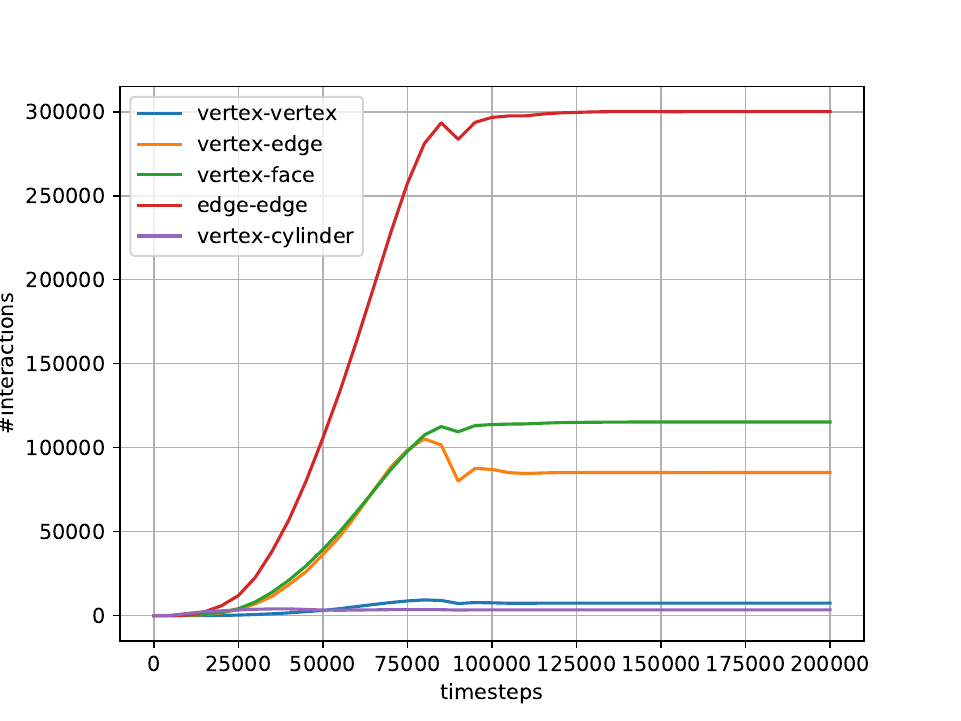
ExaDEM also offers post-processing scripts for basic interaction analyses. The scripts can be used as a basis for developing other analyses according to need. The first available script is interaction_summary.py :
Read all interaction files
Plot the number of interactions per type as a function of the timestep (types.pdf)
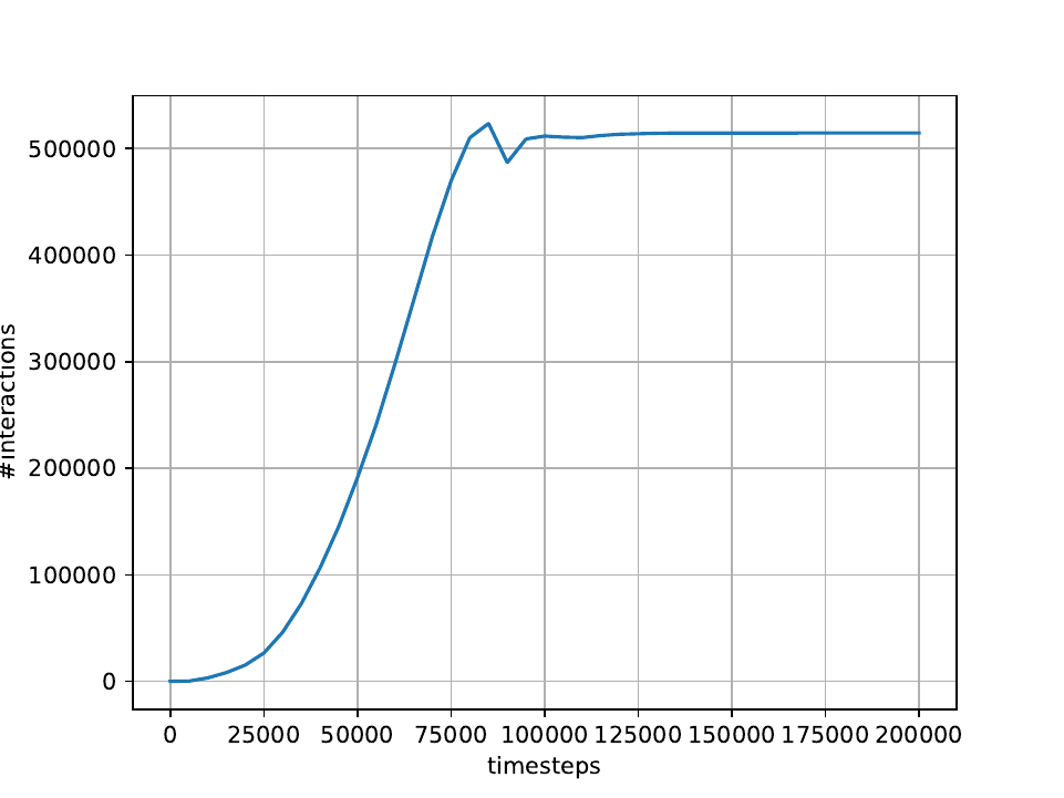
Plot the number of interactions as a function of the timestep (count.pdf)
How to run this script:
cd ExaDEMOutputDir/ExaDEMAnalyses
python3 PATH_TO_ExaDEM/scripts/post_processing/interaction_summary.py
Output file examples:
Simulation: near 104,000 octahedral particles over 200,000 timesteps of 5.10^{-5} s falling into a cylinder.
types.pdf
Note
Symmetrized interactions are counted twice within the interaction_summary.py python script.
count.pdf
4.8.6. Interaction Summary
This operator allows displaying the total number of interactions, both total and active. An interaction is considered active if there is contact and, consequently, if the cumulative friction is different from Vec3d{0,0,0}. It also enables the separation of different types of interactions: Vertex-Vertex, Vertex-Edge, Vertex-Face, and Edge-Edge.
Name: stats_interactions
No parameter.
Tip: Add this operator when performing recurring but infrequent operations such as Paraview outputs or checkpoint output files (see YAML example).
YAML example:
+dump_data_paraview:
  - stats_interactions
Output example:
=====================================================
* Type of interaction      = active / total / ghost
* Number of interactions   = 369404 / 369404 / 0
* Vertex - Vertex          = 41623 / 41623 / 0
* Vertex - Edge            = 85161 / 85161 / 0
* Vertex - Face            = 21997 / 21997 / 0
* Edge   - Edge            = 23922 / 23922 / 0
* Vertex - Cylinder        = 0 / 0 / 0
* Vertex - Surface         = 3770 / 3770 / 0
* Vertex - Ball            = 0 / 0 / 0
* Vertex - Vertex (Driver) = 0 / 0 / 0
* Vertex - Edge (Driver)   = 0 / 0 / 0
* Vertex - Face (Driver)   = 0 / 0 / 0
* Edge   - Edge (Driver)   = 0 / 0 / 0
* Edge (Driver) - Vertex   = 0 / 0 / 0
* Face (Driver) - Vertex   = 0 / 0 / 0
* Vertice - Vertex (Stick) = 192931 / 192931 / 0
=====================================================
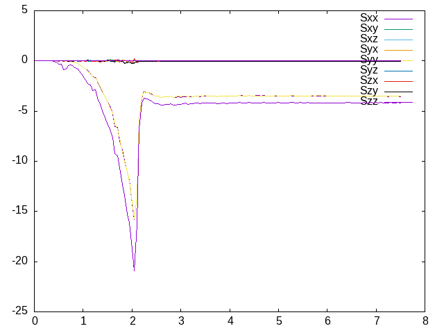
4.8.7. Global Stress Tensor
A stress tensor for a given particle is computed such as:
With I the active interactions, \(f_{ij} = (fx_{ij},fy_{ij},fz_{ij})\) the forces between the particle i and j, and \(c_{ij} = r_i - p_{ij}\) the vector between the center of the particle i noted \(r_i\) and the contact position of the interaction I named \(p_{ij}\).
And the total stress of the system : \(\sigma = \frac{1}{V} \sum_{loc} [\sigma_{loc}]\), with V the volume.
Stress tensor calculation is performed by the stress_tensor operator, and writing to a .txt output file is performed by the write_stres_tensor operator. To trigger the writing of the stress tensor, simply declare the analysis_dump_stress_tensor_frequency variable to the frequency chosen in the global operator of your YAML file (.msp), which by default is set to -1.
YAML example:
global:
  simulation_end_iteration: 150000
  simulation_log_frequency: 1000
  simulation_paraview_frequency: 10000
  analysis_dump_stress_tensor_frequency: 1000
For further information
This frequency triggers several things. When passing through the Contact Force operator, the list of interactions / normal force / tangential force is stored in the classifier. The stress tensor is then calculated in global_stress_tensor and written in write_stress_tensor. By default, volume is calculated from the simulation volume using the compute_volume operator. So, by default, the frequency will trigger the chaining of these three operators:
compute_volume:
  - domain_volume

global_stress_tensor:
  - average_stress_tensor

dump_stress_tensor_if_triggered:
  condition: trigger_write_stress_tensor
  body:
    - compute_volume
    - global_stress_tensor
    - write_stress_tensor
In the case of a particle deposit or other simulation where the simulation domain does not correspond to the simulation volume, you can either implement your my_volume operator and replace the compute_volume operator block such as:
compute_volume:
  - my_volume:
     my_param1: x
     my_param2: y
     my_param3: z
If you want to directly assign the value of a fixed-size volume, we advise you to add these lines to your input file:
compute_volume: nop

global_stress_tensor:
        - average_stress_tensor:
                 volume: 21952
A usage example is available at the following address: example/polyhedra/analyses/write_avg_stress.msp. It involves dropping a set of hexapods into a box and watching the stress tensor evolve over time.
A gnuplot script is available at scripts/post_processing/avg_stress.gnu to quickly plot lines:
set key autotitle columnhead
N = system("awk 'NR==1{print NF}' AvgStressTensor.txt")
plot for [i=2:N] "AvgStressTensor.txt" u 1:i w l
set key autotitle columnhead
set term png
set output "avgStress.png"
replot
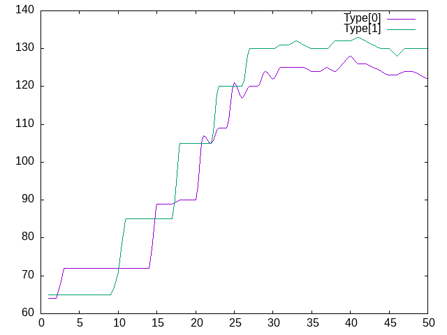
4.8.8. Particle Counter
The purpose of this operator is to count the number of particles per type in a particular region.
Operator:
Name:
particle_counterParameters:
name: Filename. Default is: ParticleCounter.txt,
types: List of particle types (required, [0,1,2, …]),
region: Choose the region, default is the domain simulation.
To use this operator, the simplest way is to define the analysis frequency (all) in the global operator (simulation_analyses_frequency) and add the particle_count operator to the operator analyses, as in the following example (see example/polyhedron/analysis/particle_counter.msp:
global:
  simulation_analyses_frequency: 10000

analyses:
  - particle_counter:
     name: "ParticleTypes0And1.txt"
     types: [0,1]
     region: BOX
One possibility for post-processing is to use gnuplot with the following commands:
set key autotitle columnheade
set style data lines
plot for [i=2:3] 'ExaDEMOutputDir/ExaDEMAnalyses/ParticleTypes0And1.txt' using 1:i smooth mcsplines
Results:
Particle Counter Output |
|
|---|---|
Simulation |
Plot |
|
|
4.8.9. Barycenter
The purpose of this operator is to count the number of particles per type in a particular region.
Operator:
Name:
particle_barycenterParameters:
name: Filename. Default is: ParticleBarycenter.txt,
types: List of particle types (required, [0,1,2, …]),
region: Choose the region, default is the domain simulation.
To use this operator, the simplest way is to define the analysis frequency (all) in the global operator (simulation_analyses_frequency) and add the particle_count operator to the operator analyses, as in the following example (see example/polyhedron/analysis/particle_barycenter.msp:
global:
  simulation_analyses_frequency: 10000

analyses:
  - particle_barycenter:
     name: BaraycenterBox.txt
     types: [0,1]
     region: BOX
  - particle_barycenter:
     name: Baraycenter.txt
     types: [0,1]
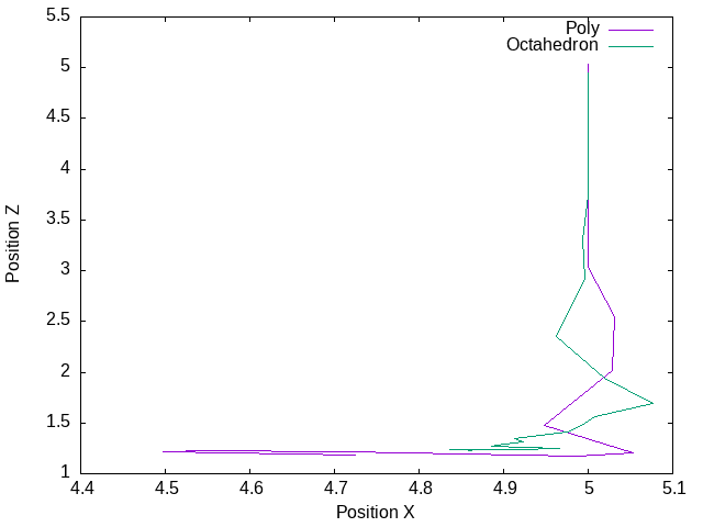
One possibility for post-processing is to use gnuplot with the following commands:
set key autotitle columnheade
set style data lines
set title font "Barycenter per particle type"
set xlabel "Position X"
set ylabel "Position Z"
plot "PolyhedraAnalysisBarycenterDir/ExaDEMAnalyses/Baraycenter.txt" u 2:4 w l title "Poly"
replot "PolyhedraAnalysisBarycenterDir/ExaDEMAnalyses/Baraycenter.txt" u 5:7 w l title "Octahedron"
set terminal png
set output "barycenter_plot.png"
replot
Particle Counter Output |
|
|---|---|
Simulation |
Plot |
|
|