Defining the domain¶

The domain operator is the primary way to fully specify a simulation domain in one block — see Alternative ways for defining the domain and Modifying the domain for other ways to set or change it afterward.

`domain`¶

Syntax

domain:
  cell_size: <float>                                       
  grid_dims: [<int>, <int>, <int>]
  bounds: [[<float>, <float>, <float>], [<float>, <float>, <float>]]
  xform: [[<float>, <float>, <float>], [<float>, <float>, <float>], [<float>, <float>, <float>]]
  periodic: [<bool>, <bool>, <bool>]
  mirror: [<string>, ...]
  expandable: <bool>

Parameters

cell_size:   float, default 0.                          # Grid cell size, in grid space.
grid_dims:   IJK, default [0,0,0]                       # 3D grid dimensions, in number of cells.
bounds:      AABB, default [[0,0,0], [0,0,0]]           # Domain bounds, in grid space.
xform:       Mat3d, default [[1,0,0],[0,1,0],[0,0,1]]   # Grid space to real space transformation matrix.
periodic:    3 booleans, default [false, false, false]  # Per-axis (x, y, z) periodic boundary conditions.
mirror:      sequence of strings, default []            # Mirrored faces — see note below for the code list.
expandable:  bool, default true                         # Allowed domain growth to keep particles.

Info

Each mirror entry is one of x, x-, x+, y, y-, y+, z, z-, z+ — a bare axis letter mirrors both faces of that axis, a signed one mirrors only that face. Setting a face's mirror disables periodicity on that axis (and vice versa).

The domain operator fully defines the simulation domain in one block: cell_size/grid_dims set the grid-space discretization, bounds/xform set the physical-space box, and periodic/mirror/expandable control boundary behavior.

Warning

All properties must be consistent with each other. In particular, cell_size multiplied by grid_dims must be equal to max(bounds) - min(bounds).

Usage examples¶

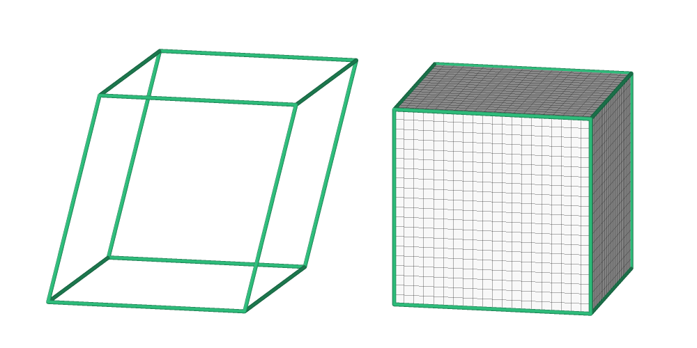
For each case below, a domain YAML block is shown alongside a visualization of the resulting physical-space and grid-space boxes.

Cubic domain¶

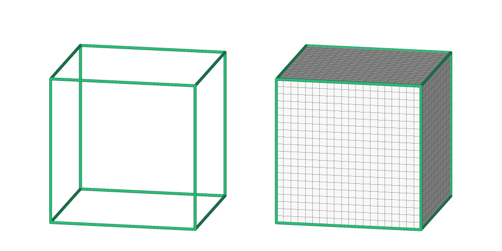
The first example creates a cubic physical domain with 100 Å side length, with 20 cells in each direction. In grid space, the domain also is cubic with the same dimensions.

domain:
  cell_size: 5.0 ang
  grid_dims: [20,20,20]
  bounds: [[0 ang ,0 ang,0 ang],[100 ang, 100 ang, 100 ang]]
  xform: [[1.,0.,0.],[0.,1.,0.],[0.,0.,1.]]
  periodic: [true,true,true]
  expandable: false

In that case, the \(\mathbf{X_f}\) matrix equals the identity matrix, so the grid-space domain is exactly equal to the physical-space domain.

Cubic domain, physical and grid space — Cubic domain, physical (left) and grid (right) space

Orthorhombic domain¶

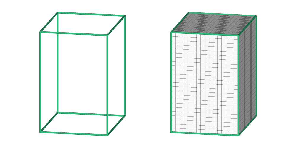
In that second example, an orthorhombic physical domain with 80 Å, 100 Å and 120 Å side lengths is created, with 16, 20 and 24 cells in each direction. In grid space, the domain is also orthorhombic with the same dimensions since the physical size exactly equals a finite number of cells in each direction.

# 1st solution
domain:
  cell_size: 5.0 ang
  grid_dims: [16,20,24]
  bounds: [[0 ang ,0 ang,0 ang],[80 ang, 100 ang, 120 ang]]
  xform: [[1.,0.,0.],[0.,1.,0.],[0.,0.,1.]]
  periodic: [true,true,true]
  expandable: false

As before, since the physical domain's size in each direction is an exact multiple of cell_size, the grid domain has the exact same dimensions.

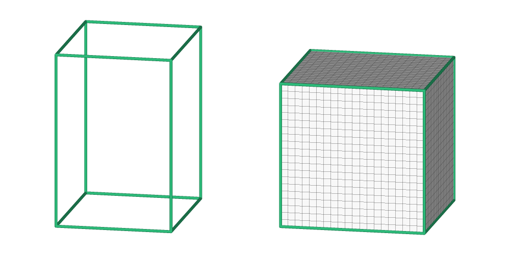
Orthorhombic domain, 1st solution, physical and grid space — Orthorhombic domain, 1st solution, physical (left) and grid (right) space

If, for some reason, the same grid dimensions are needed in each direction regardless of the physical side lengths, an orthorhombic physical domain can still be defined by choosing a non-identity \(\mathbf{X_f}\) matrix instead:

# 2nd solution
domain:
  cell_size: 5.0 ang
  grid_dims: [20,20,20]
  bounds: [[0 ang ,0 ang,0 ang],[100 ang, 100 ang, 100 ang]]
  xform: [[0.8,0.,0.],[0.,1.,0.],[0.,0.,1.2]]
  periodic: [true,true,true]
  expandable: false

This way, the physical domain has the exact same dimensions as before, but the grid domain is now cubic with 20 cells in each direction.

Orthorhombic domain, 2nd solution, physical and grid space — Orthorhombic domain, 2nd solution, physical (left) and grid (right) space

Restricted triclinic domain¶

A triclinic domain doesn't have to leave all three periodicity vectors fully free. In this example, \(\mathbf{a}\) is constrained to stay parallel to the x-axis and \(\mathbf{b}\) is confined to the \((x,y)\) plane, while \(\mathbf{c}\) remains general — a common simplification since it needs fewer independent numbers to describe the same box shape. This shows up directly in xform: it's upper triangular, with zero entries wherever a vector would otherwise pick up a component along an axis it's restricted from.

domain:
  cell_size: 5.0 ang
  grid_dims: [20,20,20]
  bounds: [[0 ang ,0 ang,0 ang],[100 ang, 100 ang, 100 ang]]
  xform: [[1.,0.1,0.2],[0.,1.,0.2],[0.,0.,1.]]
  periodic: [true,true,true]
  expandable: false

Here, \(\mathbf{a} = (1, 0, 0)\) has no \(y\) or \(z\) component and \(\mathbf{b} = (0.1, 1, 0)\) has no \(z\) component, while \(\mathbf{c} = (0.2, 0.2, 1)\) is free — exactly the constraint described above.

Restricted triclinic domain, physical and grid space — Restricted triclinic domain, physical (left) and grid (right) space

Generalized triclinic domain¶

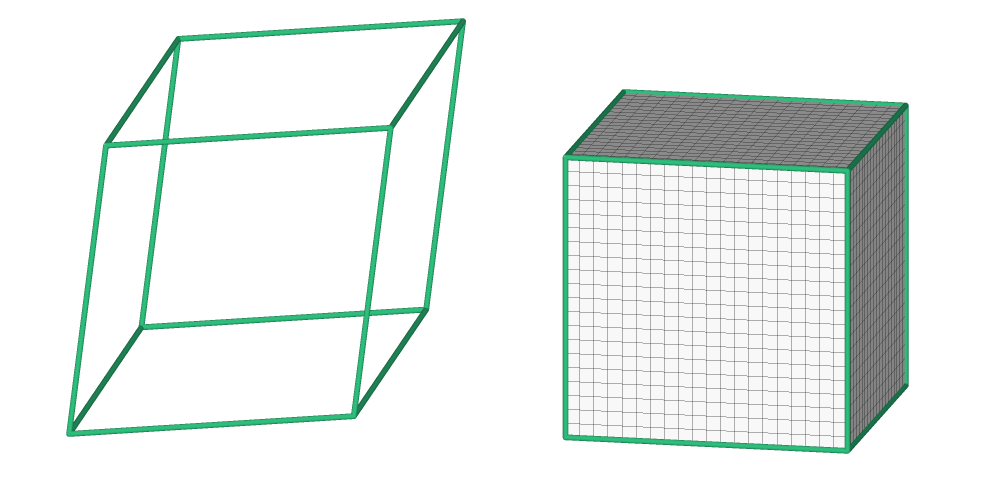
Dropping those constraints gives the fully general triclinic case: every periodicity vector can point anywhere in 3D space, so xform has no zero entries at all.

domain:
  cell_size: 5.0 ang
  grid_dims: [20,20,20]
  bounds: [[0 ang ,0 ang,0 ang],[100 ang, 100 ang, 100 ang]]
  xform: [[1.,0.05,0.1],[0.05,1.,0.1],[0.1,0.1,1.2]]
  periodic: [true,true,true]
  expandable: false

Generalized triclinic domain, physical and grid space — Generalized triclinic domain, physical (left) and grid (right) space